FIRST-ORDER PHASE TRANSITIONS
9-1 FIRST-ORDER PHASE TRANSITIONS IN SINGLE COMPONENT SYSTEMS
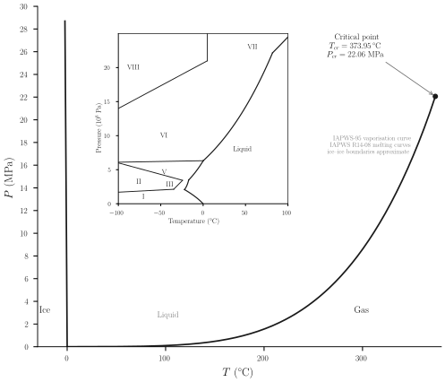
Ordinary water is liquid at room temperature and atmospheric pressure, but if cooled below 273.15 K it solidifies; and if heated above 373.15 K it vaporizes. At each of these temperatures the material undergoes a precipitous change of properties-a “phase transition.” At high pressures water undergoes several additional phase transitions from one solid form to another. These distinguishable solid phases, designated as “ice I,” “ice II,” “ice III,” … , differ in crystal structure and in essentially all thermodynamic properties (such as compressibility, molar heat capacity, and various molar potentials such as \(u\) or \(f\) ). The “phase diagram” of water is shown in Fig. 9.1.
Each transition is associated with a linear region in the thermodynamic fundamental relation (such as \(B H F\) in Fig. 8.2), and each can be viewed as the result of failure of the stability criteria (convexity or concavity) in the underlying fundamental relation.
In this section we shall consider systems for which the underlying fundamental relation is unstable. By a qualitative consideration of fluctuations in such systems we shall see that the fluctuations are profoundly influenced by the details of the underlying fundamental relation. In contrast, the average values of the extensive parameters reflect only the stable thermodynamic fundamental relation.
Consideration of the manner in which the form of the underlying fundamental relation influences the thermodynamic fluctuations will provide a physical interpretation of the stability considerations of Chapter 8 and of the construction of Fig. 8.2 (in which the thermodynamic fundamental relation is constructed as the envelope of tangent planes).
A simple mechanical model illustrates the considerations to follow by an intuitively transparent analogy. Consider a semicircular section of pipe, closed at both ends. The pipe stands vertically on a table, in the form of
an inverted U (Fig. 9.2). The pipe contains a freely-sliding internal piston separating the pipe into two sections, each of which contains one mole of a gas. The symmetry of the system will prove to have important consequences, and to break this symmetry we consider that each section of the pipe contains a small metallic “ball bearing” (i.e., a small metallic sphere). The two ball bearings are of dissimilar metals, with different coefficients of thermal expansion.
At some particular temperature, which we designate as \(T_{c}\), the two spheres have equal radii; at temperatures above \(T_{c}\) the right-hand sphere is the larger.
The piston, momentarily brought to the apex of the pipe, can fall into either of the two legs, compressing the gas in that leg and expanding the gas in the other leg. In either of these competing equilibrium states the pressure difference exactly compensates the effect of the weight of the piston.
In the absence of the two ball bearings the two competing equilibrium states would be fully equivalent. But with the ball bearings present the
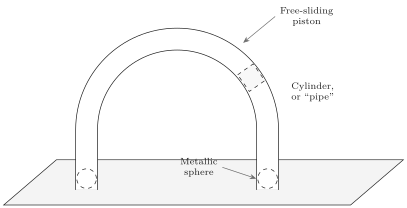
more stable equilibrium position is that to the left if \(T>T_{c}\), and it is that to the right if \(T<T_{c}\).
From a thermodynamic viewpoint the Helmholtz potential of the system is \(F=U-T S\), and the energy \(U\) contains the gravitational potential energy of the piston as well as the familiar thermodynamic energies of the two gases (and, of course, the thermodynamic energies of the two ball bearings, which we assume to be small and/or equal). Thus the Helmholtz potential of the system has two local minima, the lower minimum corresponding to the piston being on the side of the smaller sphere.
As the temperature is lowered through \(T_{c}\) the two minima of the Helmholtz potential shift, the absolute minimum changing from the left-hand to the right-hand side.
A similar shift of the equilibrium position of the piston from one side to the other can be induced at a given temperature by tilting the table-or, in the thermodynamic analogue, by adjustment of some thermodynamic parameter other than the temperature.
The shift of the equilibrium state from one local minimum to the other constitutes a first-order phase transition, induced either by a change in temperature or by a change in some other thermodynamic parameter.
The two states between which a first-order phase transition occurs are distinct, occurring at separate regions of the thermodynamic configuration space.
To anticipate “critical phenomena” and “second-order phase transitions” (Chapter 10) it is useful briefly to consider the case in which the ball bearings are identical or absent. Then at low temperatures the two competing minima are equivalent. However as the temperature is increased the two equilibrium positions of the piston rise in the pipe, approaching the apex. Above a particular temperature \(T_{c r}\), there is only one equilibrium position, with the piston at the apex of the pipe. Inversely, lowering the temperature from \(T>T_{c r}\) to \(T<T_{c r}\), the single equilibrium state bifurcates into two (symmetric) equilibrium states. The temperature \(T_{c r}\) is the “critical tempelature,” and the transition at \(T_{c r}\) is a “second-order phase transition.”
The states between which a second-order phase transition occurs are contiguous states in the thermodynamic configuration space.
In this chapter we consider first-order phase transitions. Second-order transitions will be discussed in Chapter 10. We shall there also consider the “mechanical model” in quantitative detail, whereas we here discuss it only qualitatively.
Returning to the case of dissimilar spheres, consider the piston residing in the higher minimum-that is, in the same side of the pipe as the larger ball bearing. Finding itself in such a minimum of the Helmholtz potential, the piston will remain temporarily in that minimum though undergoing thermodynamic fluctuations (“Brownian motion”). After a sufficiently long time a giant fluctuation will carry the piston “over the top” and into the stable minimum. It then will remain in this deeper minimum until an even larger (and enormously less probable) fluctuation takes it back to the less stable minimum, after which the entire scenario is repeated. The probability of fluctuations falls so rapidly with increasing amplitude (as we shall see in Chapter 19) that the system spends almost all of its time in the more stable minimum. All of this dynamics is ignored by macroscopic thermodynamics, which concerns itself only with the stable equilibrium state.
To discuss the dynamics of the transition in a more thermodynamic context it is convenient to shift our attention to a familiar thermodynamic system that again has a thermodynamic potential with two local minimum separated by an unstable intermediate region of concavity. Specifically we consider a vessel of water vapor at a pressure of 1 atm and at a temperature somewhat above 373.15 K (i.e., above the “normal boiling point” of water). We focus our attention on a small subsystem-a spherical region of such a (variable) radius that at any instant it contains one milligram of water. This subsystem is effectively in contact with a thermal reservoir and a pressure reservoir, and the condition of equilibrium is that the Gibbs potential \(G(T, P, N)\) of the small subsystem be minimum. The two independent variables which are determined by the equilibrium conditions are the energy \(U\) and the volume \(V\) of the subsystem.
If the Gibbs potential has the form shown in Fig. 9.3, where \(X_{j}\) is the volume, the system is stable in the lower minimum. This minimum corresponds to a considerably larger volume (or a smaller density) than does the secondary local minimum.
Consider the behavior of a fluctuation in volume. Such fluctuations occur continually and spontaneously. The slope of the curve in Fig. 9.3 represents an intensive parameter (in the present case a difference in pressure) which acts as a restoring “force” driving the system back toward density homogeneity in accordance with Le Chatelier’s principle. Occa-
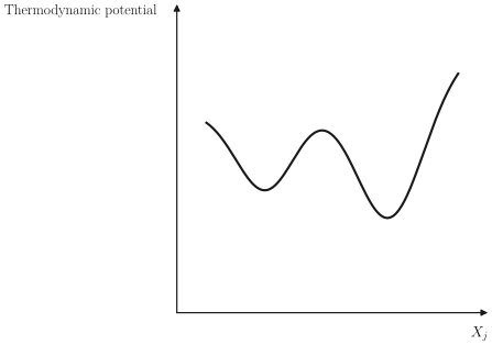
sionally a fluctuation may be so large that it takes the system over the maximum, to the region of the secondary minimum. The system then settles in the region of this secondary minimum-but only for an instant. A relatively small (and therefore much more frequent) fluctuation is all that is required to overcome the more shallow barrier at the secondary minimum. The system quickly returns to its stable state. Thus very small droplets of high density (liquid phase!) occasionally form in the gas, live briefly, and evanesce.
If the secondary minimum were far removed from the absolute minimum, with a very high intermediate barrier, the fluctuations from one minimum to another would be very improbable. In Chapter 19 it will be shown that the probability of such fluctuations decreases exponentially with the height of the intermediate free-energy barrier. In solid systems (in which interaction energies are high) it is not uncommon for multiple minima to exist with intermediate barriers so high that transitions from one minimum to another take times on the order of the age of the universe! Systems trapped in such secondary “metastable” minima are effectively in stable equilibrium (as if the deeper minimum did not exist at all).
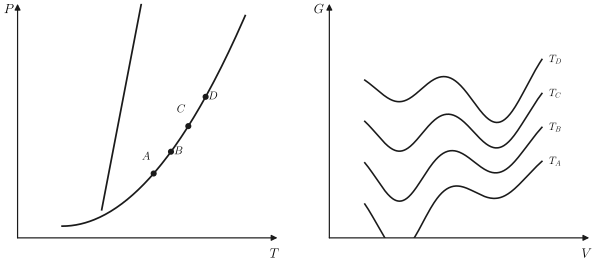
Returning to the case of water vapor at temperatures somewhat above the “boiling point,” let us suppose that we lower the temperature of the entire system. The form of the Gibbs potential varies as shown schematically in Fig. 9.4. At the temperature \(T_{4}\) the two minima become equal, and below this temperature the high density (liquid) phase becomes absolutely stable. Thus \(T_{4}\) is the temperature of the phase transition (at the prescribed pressure).
If the vapor is cooled very gently through the transition temperature the system finds itself in a state that had been absolutely stable but that is now metastable. Sooner or later a fluctuation within the system will “discover” the truly stable state, forming a nucleus of condensed liquid. This nucleus then grows rapidly, and the entire system suddenly undergoes the transition. In fact the time required for the system to discover the
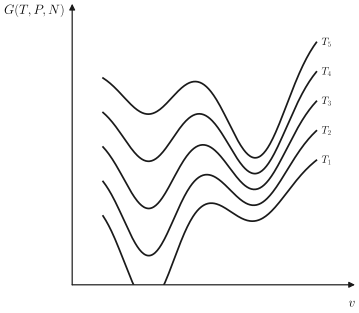
preferable state by an “exploratory” fluctuation is unobservably short in the case of the vapor to liquid condensation. But in the transition from liquid to ice the delay time is easily observed in a pure sample. The liquid so cooled below its solidification (freezing) temperature is said to be “supercooled.” A slight tap on the container, however, sets up longitudinal waves with alternating regions of “condensation” and “rarefaction,” and these externally induced fluctuations substitute for spontaneous fluctuations to initiate a precipitous transition.
A useful perspective emerges when the values of the Gibbs potential at each of its minima are plotted against temperature. The result is as shown schematically in Fig. 9.5. If these minimum values were taken from Fig. 9.4 there would be only two such curves, but any number is possible. At equilibrium the smallest minimum is stable, so the true Gibbs potential is the lower envelope of the curves shown in Fig. 9.5. The discontinuities in the entropy (and hence the latent heat) correspond to the discontinuities in slope of this envelope function.
Figure 9.5 should be extended into an additional dimension, the additional coordinate \(P\) playing a role analogous to \(T\). The Gibbs potential is then represented by the lower envelope surface, as each of the three
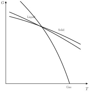
single-phase surfaces intersect. The projection of these curves of intersection onto the \(P-T\) plane is the now familiar phase diagram (e.g., Fig. 9.1).
A phase transition occurs as the state of the system passes from one envelope surface, across an intersection curve, to another envelope surface.
The variable \(X_{j}\), or \(V\) in Fig. 9.4, can be any extensive parameter. In a transition from paramagnetic to ferromagnetic phases \(X_{j}\) is the magnetic moment. In transitions from one crystal form to another (e.g., from cubic to hexagonal) the relevant parameter \(X_{j}\) is a crystal symmetry variable. In a solubility transition it may be the mole number of one component. We shall see examples of such transitions subsequently. All conform to the general pattern described.
At a first-order phase transition the molar Gibbs potential of the two phases are equal, but other molar potentials ( \(u, f, h\), etc.) are discontinuous across the transition, as are the molar volume and the molar entropy. The two phases inhabit different regions in “thermodynamic space,” and equality of any property other than the Gibbs potential would be a pure coincidence. The discontinuity in the molar potentials is the defining property of a first-order transition.
As shown in Fig. 9.6, as one moves along the liquid-gas coexistence curve away from the solid phase (i.e., toward higher temperature), the discontinuities in molar volume and molar energy become progressively smaller. The two phases become more nearly alike. Finally, at the terminus of the liquid-gas coexistence curve, the two phases become indistinguishable. The first-order transition degenerates into a more subtle transition, a second-order transition, to which we shall return in Chapter 10. The terminus of the coexistence curve is called a critical point.
The existence of the critical point precludes the possibility of a sharp distinction between the generic term liquid and the generic term gas. In crossing the liquid-gas coexistence curve in a first-order transition we distinguish two phases, one of which is “clearly” a gas and one of which is
“clearly” a liquid. But starting at one of these (say the liquid, immediately above the coexistence curve) we can trace an alternate path that skirts around the critical point and arrives at the other state (the “gas”) without ever encountering a phase transition! Thus the terms gas and liquid have more intuitive connotation than strictly defined denotation. Together liquids and gases constitute the fluid phase. Despite this we shall follow the standard usage and refer to “the liquid phase” and “the gaseous phase” in a liquid-gas first-order transition.
There is another point of great interest in Fig. 9.1: the opposite terminus of the liquid-gas coexistence curve. This point is the coterminus of three coexistence curves, and it is a unique point at which gaseous, liquid, and solid phases coexist. Such a state of three-phase compatibility is a “triple point”-in this case the triple point of water. The uniquely defined temperature of the triple point of water is assigned the (arbitrary) value of 273.16 K to define the Kelvin scale of temperature (recall Section 2.6).
PROBLEM
Problem 9.1-1
The slopes of all three curves in Fig. 9.5 are shown as negative. Is this necessary? Is there a restriction on the curvature of these curves?
9-2 THE DISCONTINUITY IN THE ENTROPY-LATENT HEAT
Phase diagrams, such as Fig. 9.1, are divided by coexistence curves into regions in which one or another phase is stable. At any point on such a curve the two phases have precisely equal molar Gibbs potentials, and both phases can coexist.
Consider a sample of water at such a pressure and temperature that it is in the “ice” region of Fig. 9.1a. To increase the temperature of the ice one must supply roughly \(2.1 \mathrm{~kJ} / \mathrm{kg}\) for every kelvin of temperature increase (the specific heat capacity of ice). If heat is supplied at a constant rate the temperature increases at an approximately constant rate. But when the temperature reaches the “melting temperature,” on the solid-liquid coexistence line, the temperature ceases to rise. As additional heat is supplied ice melts, forming liquid water at the same temperature. It requires roughly 335 kJ to melt each kg of ice. At any moment the amount of liquid water in the container depends on the quantity of heat that has entered the container since the arrival of the system at the coexistence curve (i.e., at the melting temperature). When finally the requisite amount of heat has been supplied, and the ice has been entirely melted, continued heat input again results in an increase in temperature-now at a rate determined by the specific heat capacity of liquid water ( \(\simeq 4.2 \mathrm{~kJ}\) / kg-K).
The quantity of heat required to melt one mole of solid is the heat of fusion (or the latent heat of fusion). It is related to the difference in molar entropies of the liquid and the solid phase by
\[ \ell_{L S}=T\left[s^{(L)}-s^{(S)}\right] \]
where \(T\) is the melting temperature at the given pressure. More generally, the latent heat in any first-order transition is
\[ \ell=T \Delta s \]
where \(T\) is the temperature of the transition and \(\Delta s\) is the difference in molar entropies of the two phases. Alternatively, the latent heat can be written as the difference in the molar enthalpies of the two phases
\[ \ell=\Delta h \]
which follows immediately from the identity \(h=T s+\mu\) (and the fact that \(\mu\), the molar Gibbs function, is equal in each phase). The molar enthalpies of each phase are tabulated for very many substances.
If the phase transition is between liquid and gaseous phases the latent heat is called the heat of vaporization, and if it is between solid and gaseous phases it is called the heat of sublimation.
At a pressure of one atmosphere the liquid-gas transition (boiling) of water occurs at 373.15 K, and the latent heat of vaporization is then 40.7 kJ/mole (540 cal/g).
In each case the latent heat must be put into the system as it makes a transition from the low-temperature phase to the high-temperature phase. Both the molar entropy and the molar enthalpy are greater in the high-temperature phase than in the low-temperature phase.
It should be noted that the method by which the transition is induced is irrelevant-the latent heat is independent thereof. Instead of heating the ice at constant pressure (crossing the coexistence curve of Fig. 9.1a “horizontally”), the pressure could be increased at constant temperature (crossing the coexistence curve “vertically”). In either case the same latent heat would be drawn from the thermal reservoir.
The functional form of the liquid-gas coexistence curve for water is given in “saturated steam tables”-the designation “saturated” denoting that the steam is in equilibrium with the liquid phase. (“Superheated steam tables” denote compilations of the properties of the vapor phase alone, at temperatures above that on the coexistence curve at the given pressure). An example of such a saturated steam table is given in Table 9.1, from Sonntag and Van Wylen. The properties \(s, u, v\) and \(h\) of each
ABLE 9.1 Steam Table”; Properties of the Gaseous and Liquid Phases on the Coexistence Curve of Water \({ }^{a}\)
| emp. C | Press. kPa \(P\) | Specific Volume | Internal Energy | Enthalpy | Entropy | |||||||
|---|---|---|---|---|---|---|---|---|---|---|---|---|
| Sat. Liquid \(v_{f}\) | Sat. Vapor \(v_{g}\) | Sat. Liquid \(u_{f}\) | Evap. \(u_{f g}\) | Sat. Vapor \(u_{g}\) | Sat. Liquid \(h_{f}\) | Evap. \(h_{f g}\) | Sat. Vapor \(h_{g}\) | Sat. Liquid \(s_{f}\) | Evap. \(s_{f g}\) | Sat. Vapor \(s_{g}\) | ||
| . 01 | 0.6113 | 0.001000 | 206.14 | . 00 | 2375.3 | 2375.3 | . 01 | 2501.3 | 2501.4 | . 0000 | 9.1562 | 9.1562 |
| 5 | 0.8721 | 0.001000 | 147.12 | 20.97 | 2361.3 | 2382.3 | 20.98 | 2489.6 | 2510.6 | . 0761 | 8.9496 | 9.0257 |
| 10 | 1.2276 | 0.001000 | 106.38 | 42.00 | 2347.2 | 2389.2 | 42.01 | 2477.7 | 2519.8 | . 1510 | 8.7498 | 8.9008 |
| 15 | 1.7051 | 0.001001 | 77.93 | 62.99 | 2333.1 | 2396.1 | 62.99 | 2465.9 | 2528.9 | . 2245 | 8.5569 | 8.7814 |
| 20 | 2.339 | 0.001002 | 57.79 | 83.95 | 2319.0 | 2402.9 | 83.96 | 2454.1 | 2538.1 | . 2966 | 8.3706 | 8.6672 |
| 25 | 3.169 | 0.001003 | 43.36 | 104.88 | 2304.9 | 2409.8 | 104.89 | 2442.3 | 2547.2 | . 3674 | 8.1905 | 8.5580 |
| 30 | 4.246 | 0.001004 | 32.89 | 125.78 | 2290.8 | 2416.6 | 125.79 | 2430.5 | 2556.3 | . 4369 | 8.0164 | 8.4533 |
| 35 | 5.628 | 0.001006 | 25.22 | 146.67 | 2276.7 | 2423.4 | 146.68 | 2418.6 | 2565.3 | . 5053 | 7.8478 | 8.3531 |
| 40 | 7.384 | 0.001008 | 19.52 | 167.56 | 2262.6 | 2430.1 | 167.57 | 2406.7 | 2574.3 | . 5725 | 7.6845 | 8.2570 |
| 45 | 9.593 | 0.001010 | 15.26 | 188.44 | 2248.4 | 2436.8 | 188.45 | 2394.8 | 2583.2 | . 6387 | 7.5261 | 8.1648 |
| 50 | 12.349 | 0.001012 | 12.03 | 209.32 | 2234.2 | 2443.5 | 209.33 | 2382.7 | 2592.1 | . 7038 | 7.3725 | 8.0763 |
| 55 | 15.758 | 0.001015 | 9.568 | 230.21 | 2219.9 | 2450.1 | 230.23 | 2370.7 | 2600.9 | . 7679 | 7.2234 | 7.9913 |
| 60 | 19.940 | 0.001017 | 7.671 | 251.11 | 2205.5 | 2456.6 | 251.13 | 2358.5 | 2609.6 | . 8312 | 7.0784 | 7.9096 |
| 65 | 25.03 | 0.001020 | 6.197 | 272.02 | 2191.1 | 2463.1 | 272.06 | 2346.2 | 2618.3 | . 8935 | 6.9375 | 7.8310 |
| 70 | 31.19 | 0.001023 | 5.042 | 292.95 | 2176.6 | 2469.6 | 292.98 | 2333.8 | 2626.8 | . 9549 | 6.8004 | 7.7553 |
| 75 | 38.58 | 0.001026 | 4.131 | 313.90 | 2162.0 | 2475.9 | 313.93 | 2321.4 | 2635.3 | 1.0155 | 6.6669 | 7.6824 |
| 80 | 47.39 | 0.001029 | 3.407 | 334.86 | 2147.4 | 2482.2 | 334.91 | 2308.8 | 2643.7 | 1.0753 | 6.5369 | 7.6122 |
| 85 | 57.83 | 0.001033 | 2.828 | 355.84 | 2132.6 | 2488.4 | 355.90 | 2296.0 | 2651.9 | 1.1343 | 6.4102 | 7.5445 |
| 90 | 70.14 | 0.001036 | 2.361 | 376.85 | 2117.7 | 2494.5 | 376.92 | 2283.2 | 2660.1 | 1.1925 | 6.2866 | 7.4791 |
| 95 | 84.55 | 0.001040 | 1982 | 397.88 | 2102.7 | 2500.6 | 397.96 | 2270.2 | 2668.1 | 1.2500 | 6.1659 | 74159 |
| Press. in MPa | ||||||||||||
|---|---|---|---|---|---|---|---|---|---|---|---|---|
| 100 | 0.10135 | 0.001044 | 1.6729 | 418.94 | 2087.6 | 2506.5 | 419.04 | 2257.0 | 2676.1 | 1.3069 | 6.0480 | 7.3549 |
| 105 | 0.12082 | 0.001048 | 1.4194 | 440.02 | 2072.3 | 2512.4 | 440.15 | 2243.7 | 2683.8 | 1.3630 | 5.9328 | 7.2958 |
| 110 | 0.14327 | 0.001052 | 1.2102 | 461.14 | 2057.0 | 2518.1 | 461.30 | 2230.2 | 2691.5 | 1.4185 | 5.8202 | 7.2387 |
| 115 | 0.16906 | 0.001056 | 1.0366 | 482.30 | 2041.4 | 2523.7 | 482.48 | 2216.5 | 2699.0 | 1.4734 | 5.7100 | 7.1833 |
| 120 | 0.19853 | 0.001060 | 0.8919 | 503.50 | 2025.8 | 25?9.3 | 503.71 | 2202.6 | 2706.3 | 1.5276 | 5.6020 | 7.1296 |
| 125 | 0.2321 | 0.001065 | 0.7706 | 524.74 | 2009.9 | 2634.6 | 524.99 | 2188.5 | 2713.5 | 1.5813 | 5.4962 | 7.0775 |
| 130 | 0.2701 | 0.001070 | 0.6685 | 546.02 | 1993.9 | 2539.9 | 546.31 | 2174.2 | 2720.5 | 1.6344 | 5.3925 | 7.0269 |
| 135 | 0.3130 | 0.001075 | 0.5822 | 567.35 | 1977.7 | 2545.0 | 567.69 | 2159.6 | 2727.3 | 1.6870 | 5.2907 | 6.9777 |
| 140 | 0.3613 | 0.001080 | 0.5089 | 588.74 | 1961.3 | 2550.0 | 589.13 | 2144.7 | 2733.9 | 1.7391 | 5.1908 | 6.9299 |
| 145 | 0.4154 | 0.001085 | 0.4463 | 610.18 | 1944.7 | 2554.9 | 610.63 | 2129.6 | 2740.3 | 1.7907 | 5.0926 | 6.8833 |
| 150 | 0.4758 | 0.001091 | 0.3928 | 631.68 | 1927.9 | 2559.5 | 632.20 | 2114.3 | 2746.5 | 1.8418 | 4.9960 | 6.8379 |
| 155 | 0.5431 | 0.001096 | 0.3468 | 653.24 | 1910.8 | 2564.1 | 653.84 | 2098.6 | 2752.4 | 1.8925 | 4.9010 | 6.7935 |
| 160 | 0.6178 | 0.001102 | 0.3071 | 674.87 | 1893.5 | 2568.4 | 675.55 | 2082.6 | 2758.1 | 1.9427 | 4.8075 | 6.7502 |
| 165 | 0.7005 | 0.001108 | 0.2727 | 696.56 | 1876.0 | 2572.5 | 697.34 | 2066.2 | 2763.5 | 1.9925 | 4.7153 | 6.7078 |
| 170 | 0.7917 | 0.001114 | 0.2428 | 718.33 | 1858.1 | 2576.5 | 719.21 | 2049.5 | 2768.7 | 2.0419 | 4.6244 | 6.6663 |
| 175 | 0.8920 | 0.001121 | 0.2168 | 740.17 | 1840.0 | 2580.2 | 741.17 | 2032.4 | 2773.6 | 2.0909 | 4.5347 | 6.6256 |
| 180 | 1.0021 | 0.001127 | 0.19405 | 762.09 | 1821.6 | 2583.7 | 763.22 | 2015.0 | 2778.2 | 2.1396 | 4.4461 | 6.5857 |
| 185 | 1.1227 | 0.001134 | 0.17909 | 784.10 | 1802.9 | 2587.0 | 785.37 | 1997.1 | 2782.4 | 2.1879 | 4.3586 | 6.5465 |
| 190 | 1.2544 | 0.001141 | 0.15654 | 806.19 | 1783.8 | 2590.0 | 807.62 | 1978.8 | 2786.4 | 2.2359 | 4.2720 | 6.5079 |
| 195 | 1.3978 | 0.001149 | 0.14105 | 828.37 | 1764.4 | 2592.8 | 829.98 | 1960.0 | 2790.0 | 2.2835 | 4.1863 | 6.4698 |
| 200 | 1.5538 | 0.001157 | 0.12736 | 850.65 | 1744.7 | 2595.3 | 852.45 | 1940.7 | 2793.2 | 2.3309 | 4.1014 | 6.4323 |
| 205 | 1.7230 | 0.001164 | 0.11521 | 873.04 | 1724.5 | 2597.5 | 875.04 | 1921.0 | 2796.0 | 2.3780 | 4.0172 | 6.3952 |
| 210 | 1.9062 | 0.001173 | 0.10441 | 895.53 | 1703.9 | 2599.5 | 897.76 | 1900.7 | 2798.5 | 2.4248 | 3.9337 | 6.3585 |
| 215 | 2.104 | 0.001181 | 0.09479 | 918.14 | 1682.9 | 2601.1 | 920.62 | 1879.9 | 2800.5 | 2.4714 | 3.8507 | 6.3221 |
TABLE 9.1 (continued)
| Temp. \({ }^{\circ} C T\) | Press. MPa \(P\) | Specific Volume | Internal Energy | Enthalpy | Entropy | |||||||
|---|---|---|---|---|---|---|---|---|---|---|---|---|
| Sat. Liquid \(v_{f}\) | Sat. Vapor \(v_{g}\) | Sat. Liquid \(u_{f}\) | Evap. \(u_{f g}\) | Sat. Vapor \(u_{g}\) | Sat. Liquid \(h_{f}\) | Evap. \(h_{f g}\) | Sat. Vapor \(h_{g}\) | Sat. Liquid \(s_{f}\) | Evap. \(s_{f g}\) | Sat. Vapor \(s_{g}\) | ||
| 220 | 2.318 | 0.001190 | 0.08619 | 940.87 | 1661.5 | 2602.4 | 943.62 | 1858.5 | 2802.1 | 2.5178 | 3.7683 | 6.2861 |
| 225 | 2.548 | 0.001199 | 0.07849 | 963.73 | 1639.6 | 2603.3 | 966.78 | 1836.5 | 2803.3 | 2.5639 | 3.6863 | 6.2503 |
| 230 | 2.795 | 0.001209 | 0.07158 | 986.74 | 1617.2 | 2603.9 | 990.12 | 1813.8 | 2804.0 | 2.6099 | 3.6047 | 6.2146 |
| 235 | 3.060 | 0.001219 | 0.06537 | 1009.89 | 1594.2 | 2604.1 | 1013.62 | 1790.5 | 2804.2 | 2.6558 | 3.5233 | 6.1791 |
| 240 | 3.344 | 0.001229 | 0.05976 | 1033.21 | 1570.8 | 2604.0 | 1037.32 | 1766.5 | 2803.8 | 2.7015 | 3.4422 | 6.1437 |
| 245 | 3.648 | 0.001240 | 0.05471 | 1056.71 | 1546.7 | 2603.4 | 1061.23 | 1741.7 | 2803.0 | 2.7472 | 3.3612 | 6.1083 |
| 250 | 3.973 | 0.001251 | 0.05013 | 1080.39 | 1522.0 | 2602.4 | 1085.36 | 1716.2 | 2801.5 | 2.7927 | 3.2802 | 6.0730 |
| 255 | 4.319 | 0.001263 | 0.04598 | 1104.28 | 1496.7 | 2600.9 | 1109.73 | 1689.8 | 2799.5 | 2.8383 | 3.1992 | 6.0375 |
| 260 | 4.688 | 0.001276 | 0.04221 | 1128.39 | 1470.6 | 2599.0 | 1134.37 | 1662.5 | 2796.9 | 2.8838 | 3.1181 | 6.0019 |
| 265 | 5.081 | 0.001289 | 0.03877 | 1152.74 | 1443.9 | 2596.6 | 1159.28 | 1634.4 | 2793.6 | 2.9294 | 3.0368 | 5.9662 |
| 270 | 5.499 | 0.001302 | 0.03564 | 1177.36 | 1416.3 | 2593.7 | 1184.51 | 1605.2 | 2789.7 | 2.9751 | 2.9551 | 5.9301 |
| 275 | 5.942 | 0.001317 | 0.03279 | 1202.25 | 1387.9 | 2590.2 | 1210.07 | 1574.9 | 2785.0 | 3.0208 | 2.8730 | 5.8938 |
| 280 | 6.412 | 0.001332 | 0.03017 | 1227.46 | 1358.7 | 2586.1 | 1235.99 | 1543.6 | 2779.6 | 3.0668 | 2.7903 | 5.8571 |
| 285 | 6.909 | 0.001348 | 0.02777 | 1253.00 | 1328.4 | 2581.4 | 1262.31 | 1511.0 | 2773.3 | 3.1130 | 2.7070 | 5.8199 |
| 290 | 7.436 | 0.001366 | 0.02557 | 1278.92 | 1297.1 | 2576.0 | 1289.07 | 1477.1 | 2766.2 | 3.1594 | 2.6227 | 5.7821 |
| 295 | 7.993 | 0.001384 | 0.02354 | 1305.2 | 1264.7 | 2569.9 | 1316.3 | 1441.8 | 2758.1 | 3.2062 | 2.5375 | 5.7437 |
| 300 | 8.581 | 0.001404 | 0.02167 | 1332.0 | 1231.0 | 2563.0 | 1344.0 | 1404.9 | 2749.0 | 3.2534 | 2.4511 | 5.7045 |
| 305 | 9.202 | 0.001425 | 0.019948 | 1359.3 | 1195.9 | 2555.2 | 1372.4 | 1366.4 | 2738.7 | 3.3010 | 2.3633 | 5.6643 |
| 310 | 9.856 | 0.001447 | 0.018350 | 1387.1 | 1159.4 | 2546.4 | 1401.3 | 1326.0 | 2727.3 | 3.3493 | 2.2737 | 5.6230 |
| 315 | 10.547 | 0.001472 | 0.016867 | 1415.5 | 1121.1 | 2536.6 | 1431.0 | 1283.5 | 2714.5 | 3.3982 | 2.1821 | 5.5804 |
|---|---|---|---|---|---|---|---|---|---|---|---|---|
| 320 | 11.274 | 0.001499 | 0.015488 | 1444.6 | 1080.9 | 2525.5 | 1461.5 | 1238.6 | 2700.1 | 3.4480 | 2.0882 | 5.5362 |
| 330 | 12.845 | 0.001561 | 0.012996 | 1505.3 | 993.7 | 2498.9 | 1525.3 | 1140.6 | 2665.9 | 3.5507 | 1.8909 | 5.4417 |
| 340 | 14.586 | 0.001638 | 0.010797 | 1570.3 | 894.3 | 2464.6 | 1594.2 | 1027.9 | 2622.0 | 3.6594 | 1.6763 | 5.3357 |
| 350 | 16.513 | 0.001740 | 0.008813 | 1641.9 | 776.6 | 2418.4 | 1670.6 | 893.4 | 2563.9 | 3.7777 | 1.4335 | 5.2112 |
| 360 | 18.651 | 0.001893 | 0.006945 | 1725.2 | 626.3 | 2351.5 | 1760.5 | 720.5 | 2481.0 | 3.9147 | 1.1379 | 5.0526 |
| 370 | 21.03 | 0.002213 | 0.004925 | 1844.0 | 384.5 | 2228.5 | 1890.5 | 441.6 | 2332.1 | 4.1106 | . 6865 | 4.7971 |
| 374.14 | 22.09 | 0.003155 | 0.003155 | 2029.6 | 0 | 2029.6 | 2099.3 | 0 | 2099.3 | 4.4298 | 0 | 4.4298 |
1phase are conventionally listed in such tables; the latent heat of the transition is the difference in the molar enthalpies of the two phases, or it can also be obtained as \(T \Delta s\).
1 \({ }^{a}\) From R. E. Sonntag and G. J. Van Wylen, Introduction to Thermodynamics, Classical and Statistical”, John Wiley & Sons, New York, 1982 (adapted from J. H. Keenan, F. G. Keyes, P. G. Hill, and J. G. Moore, Steam Tables, John Wiley & Sons, New York, 1978).
Similar data are compiled in the thermophysical data literature for a wide variety of other materials.
The molar volume, like the molar entropy and the molar energy, is discontinuous across the coexistence curve. For water this is particularly interesting in the case of the solid-liquid coexistence curve. It is common experience that ice floats in liquid water. The molar volume of the solid (ice) phase accordingly is greater than the molar volume of the liquid phase-an uncommon attribute of \(\mathrm{H}_{2} \mathrm{O}\). The much more common situation is that in which the solid phase is more compact, with a smaller molar volume. One mundane consequence of this peculiar property of \(\mathrm{H}_{2} \mathrm{O}\) is the proclivity of frozen plumbing to burst. A compensating consequence, to which we shall return in Section 9.3, is the possibility of ice skating. And, underlying all, this peculiar property of water is essential to the very possibility of life on earth. If ice were more dense than liquid water the frozen winter surfaces of lakes and oceans would sink to the bottom; new surface liquid, unprotected by an ice layer, would again freeze (and sink) until the entire body of water would be frozen solid (“frozen under” instead of “frozen over”).
PROBLEMS
Problem 9.2-1
In a particular solid-liquid phase transition the point \(P_{0}, T_{0}\) lies on the coexistence curve. The latent heat of vaporization at this point is \(\ell_{0}\). A nearby point on the coexistence curve has pressure \(P_{0}+p\) and temperature \(T_{0}+t\); the local slope of the coexistence curve in the \(P-T\) plane is \(p / t\). Assuming \(v, c_{p}, \alpha\), and \(\kappa_{T}\) to be known in each phase in the vicinity of the states of interest, find the latent heat at the point \(P_{0}+p, T_{0}+t\).
Problem 9.2-2
Discuss the equilibrium that eventually results if a solid is placed in an initially evacuated closed container and is maintained at a given temperature. Explain why the solid-gas coexistence curve is said to define the “vapor pressure of the solid” at the given temperature.
9-3 THE SLOPE OF COEXISTENCE CURVES; THE CLAPEYRON EQUATION
The coexistence curves illustrated in Fig. 9.1 are less arbitrary than is immediately evident; the slope \(d P / d T\) of a coexistence curve is fully determined by the properties of the two coexisting phases.
The slope of a coexistence curve is of direct physical interest. Consider cubes of ice at equilibrium in a glass of water. Given the ambient pressure, the temperature of the mixed system is determined by the liquid-solid coexistence curve of water; if the temperature were not on the coexistence curve some ice would melt, or some liquid would freeze, until the temperature would again lie on the coexistence curve (or one phase would become depleted). At 1 atm of pressure the temperature would be 273.15 K. If the ambient pressure were to decrease-perhaps by virtue of a change in altitude (the glass of water is to be served by the flight attendant in an airplane), or by a variation in atmospheric conditions (approach of a storm)-then the temperature of the glass of water would appropriately adjust to a new point on the coexistence curve. If \(\Delta P\) were the change in pressure then the change in temperature would be \(\Delta T=\Delta P /(d P / d T)_{c c}\), where the derivative in the denominator is the slope of the coexistence curve. Ice skating, to which we have made an earlier allusion, presents another interesting example. The pressure applied to the ice directly beneath the blade of the skate shifts the ice across the solid-liquid coexistence curve (vertically upward in Fig. 9.1a), providing a lubricating film of liquid on which the skate slides. The possibility of ice skating depends on the negative slope of the liquid-solid coexistence curve of water. The existence of the ice on the upper surface of the lake, rather than on the bottom, reflects the larger molar volume of the solid phase of water as compared to that of the liquid phase. The connection of these two facts, which are not independent, lies in the Clapeyron equation, to which we now turn.
Consider the four states shown in Fig. 9.7. States \(A\) and \(A^{\prime}\) are on the coexistence curve, but they correspond to different phases (to the left-hand and right-hand regions respectively.) Similarly for the states \(B\) and \(B^{\prime}\). The pressure difference \(P_{B}-P_{A}\) (or, equivalently, \(P_{B^{\prime}}-P_{A^{\prime}}\) ) is assumed to be infinitesimal \((=d P)\), and similarly for the temperature difference \(T_{B}-T_{A}(=d T)\). The slope of the curve is \(d P / d T\).
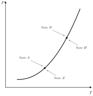
Phase equilibrium requires that
\[ \mu_{A}=\mu_{A^{\prime}} \]
and
\[ \mu_{B}=\mu_{B^{\prime}} \]
whence
\[ \mu_{B}-\mu_{A}=\mu_{B^{\prime}}-\mu_{A^{\prime}} \]
But
\[ \mu_{B}-\mu_{A}=-s d T+v d P \]
and
\[ \mu_{B^{\prime}}-\mu_{A^{\prime}}=-s^{\prime} d T+v^{\prime} d P \]
in which \(s\) and \(s^{\prime}\) are the molar entropies and \(v\) and \(v^{\prime}\) are the molar volumes in each of the phases. By inserting equations 9.7 and 9.8 in equation 9.6 and rearranging the terms, we easily find
\[ \begin{aligned} & \frac{d P}{d T}=\frac{s^{\prime}-s}{v^{\prime}-v} \\ & \frac{d P}{d T}=\frac{\Delta s}{\Delta v} \end{aligned} \]
in which \(\Delta s\) and \(\Delta v\) are the discontinuities in molar entropy and molar volume associated with the phase transition. According to equation 9.2 the latent heat is
\[ \ell=T \Delta s \]
whence
\[ \frac{d P}{d T}=\frac{\ell}{T \Delta v} \]
This is the Clapeyron equation. The Clapeyron equation embodies the Le Chatelier principle. Consider a solid-liquid transition with a positive latent heat \(\left(s_{\ell}>s_{s}\right)\) and a positive difference of molar volumes \(\left(v_{\ell}>v_{3}\right)\). The slope of the phase curve is correspondingly positive. Then an increase in pressure at constant temperature tends to drive the system to the more dense (solid) phase (alleviating the pressure increase), and an increase in temperature tends to drive the system to the more entropic (liquid) phase. Conversely, if \(s_{\ell}>s_{s}\) but \(v_{\ell}<v_{s}\), then the slope of the coexistence curve is negative, and an increase of the pressure (at constant \(T\) ) tends to drive the system to the liquid phase-again the more dense phase.
In practical problems in which the Clapeyron equation is applied it is often sufficient to neglect the molar volume of the liquid phase relative to the molar volume of the gaseous phase \(\left(v_{g}-v_{l} \simeq v_{g}\right)\), and to approximate the molar volume of the gas by the ideal gas equation \(\left(v_{g} \simeq R T / P\right)\). This “Clapeyron-Clausius approximation” may be used where appropriate in the problems at the end of this section.
Example
A light rigid metallic bar of rectangular cross section lies on a block of ice, extending slightly over each end. The width of the bar is 2 mm and the length of the bar in contact with the ice is 25 cm . Two equal masses, each of mass \(M\), are hung from the extending ends of the bar. The entire system is at atmospheric pressure and is maintained at a temperature of \(T=-2^{\circ} \mathrm{C}\). What is the minimum value of \(M\) for which the bar will pass through the block of ice by “regelation”? The given data are that the latent heat of fusion of water is 80 cal/gram, that the density of liquid water is \(1 \mathrm{gram} / \mathrm{cm}^{3}\), and that ice cubes float with \(\simeq 4 / 5\) of their volume submerged.
Solution
The Clapeyron equation permits us to find the pressure at which the solid-liquid transition occurs at \(T=-2^{\circ} \mathrm{C}\). However we must first use the “ice cube data” to obtain the difference \(\Delta v\) in molar volumes of liquid and solid phases. The data given imply that the density of ice is \(0.8 \mathrm{~g} / \mathrm{cm}^{3}\). Furthermore \(v_{\mathrm{hq}} \simeq 18 \mathrm{~cm}^{3} / \mathrm{mole}\), and therefore \(v_{\text {solid }} \simeq 22.5 \times 10^{-6} \mathrm{~m}^{3} / \mathrm{mole}\). Thus
\[ \left.\frac{d P}{d T}\right)_{c c}=\frac{\ell}{T \Delta v}=\frac{(80 \times 4.2 \times 18) \mathrm{J} / \mathrm{mole}}{271 \times\left(-4.5 \times 10^{-6}\right) \mathrm{K}-\mathrm{m}^{3} / \mathrm{mole}}=-5 \times 10^{6} \mathrm{~Pa} / \mathrm{K} \]
so that the pressure difference required is
\[ P \simeq-5 \times 10^{6} \times(-2) \simeq 10^{7} \mathrm{~Pa} \]
This pressure is to be obtained by a weight 2 Mg acting on the area \(A=5 \times 10^{-3} \mathrm{~m}^{2}\),
\[ \begin{aligned} M & =\frac{1}{2} \Delta P \frac{A}{g} \\ & =\frac{1}{2}\left(10^{7} \mathrm{~Pa}\right)\left(5 \times 10^{-5} \mathrm{~m}^{2}\right) /\left(9.8 \frac{\mathrm{~m}}{\mathrm{~s}^{2}}\right)=2.6 \mathrm{Kg} \end{aligned} \]
PROBLEMS
Problem 9.3-1
A particular liquid boils at 127°C at a pressure of 800 mm Hg. It has a heat of vaporization of \(1000 \mathrm{cal} /\) mole. At what temperature will it boil if the pressure is raised to 810 mm Hg ?
Problem 9.3-2
A long vertical column is closed at the bottom and open at the top; it is partially filled with a particular liquid and cooled to \(-5^{\circ} \mathrm{C}\). At this temperature the fluid solidifies below a particular level, remaining liquid above this level. If the temperature is further lowered to \(-5.2^{\circ} \mathrm{C}\) the solid-liquid interface moves upward by 40 cm . The latent heat (per unit mass) is \(2 \mathrm{cal} / \mathrm{g}\), and the density of the liquid phase is \(1 \mathrm{~g} / \mathrm{cm}^{3}\). Find the density of the solid phase. Neglect thermal expansion of all materials.
Hint: Note that the pressure at the original position of the interface remains constant.
Answer: \(2.6 \mathrm{~g} / \mathrm{cm}^{3}\)
Problem 9.3-3
It is found that a certain liquid boils at a temperature of 95°C at the top of a hill, whereas it boils at a temperature of \(105^{\circ} \mathrm{C}\) at the bottom. The latent heat is \(1000 \mathrm{cal} /\) mole . What is the approximate height of the hill?
Problem 9.3-4
Two weights are hung on the ends of a wire, which passes over a block of ice. The wire gradually passes through the block of ice, but the block remains intact even after the wire has passed completely through it. Explain why less mass is required if a semi-flexible wire is used, rather than a rigid bar as in the Example.
Problem 9.3-5
In the vicinity of the triple point the vapor pressure of liquid ammonia (in Pascals) is represented by
\[ \ln P=24.38-\frac{3063}{T} \]
This is the equation of the liquid-vapor boundary curve in a \(P-T\) diagram. Similarly, the vapor pressure of solid ammonia is
\[ \ln P=27.92-\frac{3754}{T} \]
What are the temperature and pressure at the triple point? What are the latent heats of sublimation and vaporization? What is the latent heat of fusion at the triple point?
Problem 9.3-6
Let \(x\) be the mole fraction of solid phase in a solid-liquid two-phase system. If the temperature is changed at constant total volume, find the rate of change of \(x\); that is, find \(d x / d T\). Assume that the standard parameters \(v\), \(\alpha, \kappa_{T}, c_{P}\) are known for each phase.
Problem 9.3-7
A particular material has a latent heat of vaporization of \(5 \times 10^{3} \mathrm{~J} /\) mole , constant along the coexistence curve. One mole of this material exists in two-phase (liquid-vapor) equilibrium in a container of volume \(V=10^{-2} \mathrm{~m}^{3}\), at a temperature of 300 K and a pressure of \(10^{5} \mathrm{~Pa}\). The system is heated at constant volume, increasing the pressure to \(2.0 \times 10^{5} \mathrm{~Pa}\). (Note that this is not a small \(\Delta P\).) The vapor phase can be treated as a monatomic ideal gas, and the molar volume of the liquid can be neglected relative to that of the gas. Find the initial and final mole fractions of the vapor phase \(\left[x \equiv N_{g} /\left(N_{g}+N_{e}\right)\right]\).
Problem 9.3-8
Draw the phase diagram, in the \(B_{e}-T\) plane, for a simple ferromagnet; assume no magnetocrystalline anisotropy and assume the external field \(B_{e}\) to be always parallel to a fixed axis in space. What is the slope of the coexistence curve? Explain this slope in terms of the Clapeyron equation.
Problem 9.3-9
A system has coexistence curves similar to those shown in Fig. 9.6a, but with the liquid-solid coexistence curve having a positive slope. Sketch the isotherms in the \(P-v\) plane for temperature \(T\) such that
- \(T<T_{t}\),
- \(T=T_{t}\),
- \(T_{t} \leq T<T_{\text {crit }}\),
- \(T_{t}<T \lesssim T_{\text {crit }}\),
- \(T=\) \(T_{\text {crit }}, \quad\) (f) \(T \geq T_{\text {crit }}\).
Here \(T_{t}\) and \(T_{\text {crit }}\) denote the triple point and critical temperatures, respectively.
9-4 UNSTABLE ISOTHERMS AND FIRST-ORDER PHASE TRANSITIONS
Our discussion of the origin of first-order phase transitions has focused, quite properly, on the multiple minima of the Gibbs potential. But although the Gibbs potential may be the fundamental entity at play, a more common description of a thermodynamic system is in terms of the form of its isotherms. For many gases the shape of the isotherms is well represented (at least semiquantitatively) by the van der Waals equation of state (recall Section 3.5)
\[ P=\frac{R T}{(v-b)}-\frac{a}{v^{2}} \]
The shape of such van der Waals isotherms is shown schematically in the \(P-v\) diagram of Fig. 9.8.
As pointed out in Section 3.5 the van der Waals equation of state can be viewed as an “underlying equation of state,” obtained by curve fitting, by inference based on plausible heuristic reasoning, or by statistical mechanical calculations based on a simple molecular model. Other empirical or semiempirical equations of state exist, and they all have isotherms that are similar to those shown in Fig. 9.8.
We now explore the manner in which isotherms of the general form shown reveal and define a phase transition.
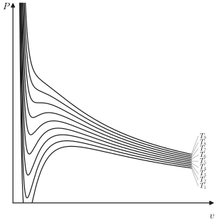
It should be noted immediately that the isotherms of Fig. 9.8 do not satisfy the criteria of intrinsic stability everywhere, for one of these criteria (equation 8.21) is \(\kappa_{T}>0\), or
\[ \left(\frac{\partial P}{\partial V}\right)_{T}<0 \]
This condition clearly is violated over the portion FKM of a typical isotherm (which, for clarity, is shown separately in Fig. 9.9). Because of this violation of the stability condition a portion of the isotherm must be unphysical, superseded by a phase transition in a manner which will be explored shortly.
The molar Gibbs potential is essentially determined by the form of the isotherm. From the Gibbs-Duhem relation we recall that
\[ d \mu=-s d T+v d P \]
whence, integrating at constant temperature
\[ \mu=\int v d P+\phi(T) \]
where \(\phi(T)\) is an undetermined function of the temperature, arising as the “constant of integration.” The integrand \(v(P)\), for constant temperature, is given by Fig. 9.9, which is most conveniently represented with \(P\) as
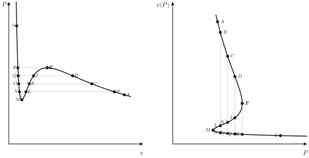
abscissa and \(v\) as ordinate. By arbitrarily assigning a value to the chemical potential at the point \(A\), we can now compute the value of \(\mu\) at any other point on the same isotherm, such as \(B\), for from equation 9.16
\[ \mu_{B}-\mu_{A}=\int_{A}^{B} v(P) d P \]
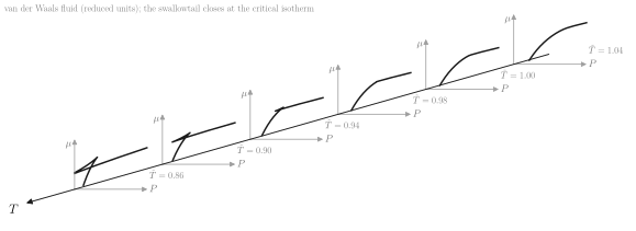
In this way we obtain Fig. 9.10. This figure, representing \(\mu\) versus \(P\), can be considered as a plane section of a three-dimensional representation of \(\mu\) versus \(P\) and \(T\), as shown in Fig. 9.11. Four different constant-temperature sections of the \(\mu\)-surface, corresponding to four isotherms, are shown. It is also noted that the closed loop of the \(\mu\) versus \(P\) curves, which results from the fact that \(v(P)\) is triple valued in \(P\) (see Fig. 9.9), disappears for high temperatures in accordance with Fig. 9.8.
Finally, we note that the relation \(\mu=\mu(T, P)\) constitutes a fundamental relation for one mole of the material, as the chemical potential \(\mu\) is the Gibbs function per mole. It would then appear from Fig. 9.11 that we have almost succeeded in the construction of a fundamental equation from a single given equation of state, but it should be recalled that although each of the traces of the \(\mu\)-surface (in the various constant temperature planes of Fig. 9.11) has the proper form, each contains an additive “constant” \(\phi(T)\), which varies from one temperature plane to another. Consequently, we do not know the complete form of the \(\mu(T, P)\)-surface, although we certainly are able to form a rather good mental picture of its essential topological properties.
With this qualitative picture of the fundamental relation implied by the van der Waals equation, we return to the question of stability.
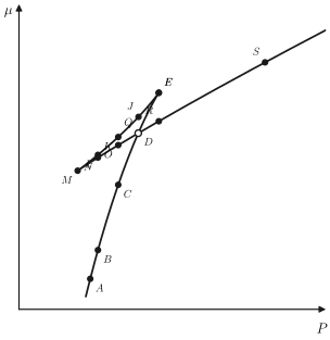
Consider a system in the state \(A\) of Fig. 9.9 and in contact with thermal and pressure reservoirs. Suppose the pressure of the reservoir to be increased quasi-statically, maintaining the temperature constant. The system proceeds along the isotherm in Fig. 9.9 from the point \(A\) in the direction of point \(B\). For pressures less than \(P_{B}\) we see that the volume of the system (for given pressure and temperature) is single valued and unique. As the pressure increases above \(P_{B}\), however, three states of equal \(P\) and \(T\) become available to the system, as, for example, the states designated by \(C, L\), and \(N\). Of these three states \(L\) is unstable, but at both \(C\) and \(N\) the Gibbs potential is a (local) minimum. These two local minimum values of the Gibbs potential (or of \(\mu\) ) are indicated by the points \(C\) and \(N\) in Fig. 9.10. Whether the system actually selects the state \(C\) or the state \(N\) depends upon which of these two local minima of the Gibbs potential is the lower, or absolute, minimum. It is clear from Fig. 9.10 that the state \(C\) is the true physical state for this value of the pressure and temperature.
As the pressure is further slowly increased, the unique point \(D\) is reached. At this point the \(\mu\)-surface intersects itself, as shown in Fig. 9.10, and the absolute minimum of \(\mu\) or \(G\) thereafter comes from the other branch of the curve. Thus at the pressure \(P_{E}=P_{Q}\), which is greater than \(P_{D}\), the physical state is \(Q\). Below \(P_{D}\) the right-hand branch of the isotherm in Fig. \(9.9 a\) is the physically significant branch, whereas above \(P_{D}\) the left-hand branch is physically significant. The physical isotherm thus deduced from the hypothetical isotherm of Fig. 9.9 is therefore shown in Fig. 9.12.
The isotherm of Fig. 9.9 belongs to an “underlying fundamental relation”; that of Fig. 9.12 belongs to the stable “thermodynamic fundamental relation.”
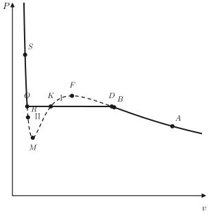
The points \(D\) and \(O\) are determined by the condition that \(\mu_{D}=\mu_{O}\) or, from equation 9.17
\[ \int_{D}^{O} v(P) d P=0 \]
where the integral is taken along the hypothetical isotherm. Referring to Fig. 9.9, we see that this condition can be given a direct graphical interpretation by breaking the integral into several portions
\[ \int_{D}^{F} v d P+\int_{F}^{K} v d P+\int_{K}^{M} v d P+\int_{M}^{O} v d P=0 \]
and rearranging as follows
\[ \int_{D}^{F} v d P-\int_{K}^{F} v d P=\int_{M}^{K} v d P-\int_{M}^{O} v d P \]
Now the integral \(\int_{D}^{F} v d P\) is the area under the arc \(D F\) in Fig. 9.12 and the integral \(\int_{K}^{F} v d P\) is the area under the arc \(K F\). The difference in these integrals is the area in the closed region \(D F K D\), or the area marked \(\mathbf{I}\) in Fig. 9.12. Similarly, the right-hand side of equation 9.20 represents the area II in Fig. 9.12, and the unique points \(O\) and \(D\) are therefore determined by the graphical condition
\[ \operatorname{area} I=\operatorname{area} I I \]
It is only after the nominal (non-monotonic) isotherm has been truncated by this equal area construction that it represents a true physical isotherm.
Not only is there a nonzero change in the molar volume at the phase transition, but there are associated nonzero changes in the molar energy and the molar entropy as well. The change in the entropy can be computed by integrating the quantity
\[ d s=\left(\frac{\partial s}{\partial v}\right)_{T} d v \]
along the hypothetical isotherm \(O M K F D\). Alternatively, by the thermodynamic mnemonic diagram, we can write
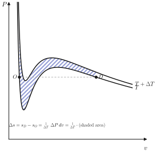
\[ \Delta s=s_{D}-s_{O}=\int_{O M K F D}\left(\frac{\partial P}{\partial T}\right)_{v} d v \]
A geometrical interpretation of this entropy difference, in terms of the area between neighboring isotherms, is shown in Fig. 9.13.
As the system is transformed at fixed temperature and pressure from the pure phase \(O\) to the pure phase \(D\), it absorbs an amount of heat per mole equal to \(l_{D O}=T \Delta s\). The volume change per mole is \(\Delta v=v_{D}-v_{O}\), and this is associated with a transfer of work equal to \(P \Delta v\). Consequently, the total change in the molar energy is
\[ \Delta u=u_{D}-u_{O}=T \Delta s-P \Delta v \]
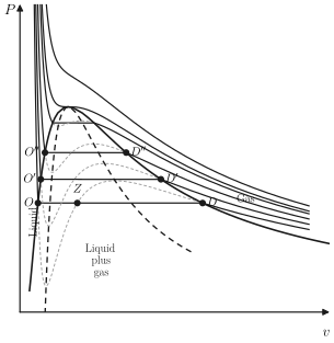
Each isotherm, such as that of Fig. 9.12, has now been classified into three regions. The region \(S O\) is in the liquid phase. The region \(D A\) is in the gaseous phase. The flat region \(O K D\) corresponds to a mixture of the two phases. Thereby the entire \(P-v\) plane is classified as to phase, as shown in Fig. 9.14. The mixed liquid-plus-gas region is bounded by the inverted parabola-like curve joining the extremities of the flat regions of each isotherm.
Within the two-phase region any given point denotes a mixture of the two phases at the extremities of the flat portion of the isotherm passing through that point. The fraction of the system that exists in each of the two phases is governed by the “lever rule.” Let us suppose that the molar volumes at the two extremities of the flat region of the isotherm are \(v_{\ell}\) and \(v_{g}\) (suggesting but not requiring that the two phases are liquid and gas, for definiteness). Let the molar volume of the mixed system be \(v=V / N\). Then if \(x_{\ell}\) and \(x_{g}\) are the mole fractions of the two phases
\[ V=N v=N x_{\ell} v_{\ell}+N x_{g} v_{g} \]
from which one easily finds
\[ x_{\ell}=\frac{v_{g}-v}{v_{g}-v_{\ell}} \]
and
\[ x_{g}=\frac{v-v_{\ell}}{v_{g}-v_{\ell}} \]
That is, an intermediate point on the flat portion of the isotherm implies a mole fraction of each phase that is equal to the fractional distance of the point from the opposite end of the flat region. Thus the point \(Z\) in Fig. 9.14 denotes a mixed liquid-gas system with a mole fraction of liquid phase equal to the “length” \(Z D\) divided by the “length” \(O D\). This is the very convenient and pictorial lever rule.
The vertex of the two-phase region, or the point at which \(O^{\prime \prime}\) and \(D^{\prime \prime}\) coincide in Fig. 9.14, corresponds to the critical point-the termination of the gas-liquid coexistence curve in Fig. 9.1a. For temperatures above the critical temperature the isotherms are monotonic (Fig. 9.14) and the molar Gibbs potential no longer is reentrant (Fig. 9.10).
Just as a \(P-v\) diagram exhibits a two-phase region, associated with the discontinuity in the molar volume, so a \(T-s\) diagram exhibits a two-phase region associated with the discontinuity in the molar entropy.
Example 1
Find the critical temperature \(T_{c r}\) and critical pressure \(P_{c r}\) for a system described by the van der Waals equation of state. Write the van der Waals equation of state in terms of the reduced variabies \(\tilde{T} \equiv T / T_{c r}, \tilde{P} \equiv P / P_{c r}\) and \(\tilde{v} \equiv v / v_{c r}\).
Solution The critical state coincides with a point of horizontal inflection of the isotherm, or
\[ \left(\frac{\partial P}{\partial v}\right)_{T_{c r}}=\left(\frac{\partial^{2} P}{\partial v^{2}}\right)_{T_{c r}}=0 . \]
(Why?) Solving these two simultaneous equations gives
\[ v_{c r}=3 b \quad P_{c r}=\frac{a}{27 b^{2}}, \quad R T_{c r}=\frac{8 a}{27 b} \]
from which we can write the van der Waals equation in reduced variables:
\[ \tilde{P}=\frac{8 \tilde{T}}{3 \tilde{v}-1}-\frac{3}{\tilde{v}^{2}} \]
Example 2
Calculate the functional form of the boundary of the two-phase region in the \(P-T\) plane for a system described by the van der Waals equation of state.
Solution We work in reduced variables, as defined in the preceding example. We consider a fixed temperature and we carry out a Gibbs equal area construction on the corresponding isotherm. Let the extremities of the two-phase region, corresponding to the reduced temperature \(\tilde{T}\), be \(\tilde{v}_{g}\) and \(\tilde{v}_{\ell}\). The equal area construction corresponding to equations 9.20 and 9.21 is
\[ \int_{v_{\ell}}^{v_{g}} \tilde{P} d \tilde{v}=\tilde{P}_{\ell}\left(\tilde{v}_{g}-\tilde{v}_{\ell}\right) \]
where \(\tilde{P}_{\ell}=\tilde{P}_{g}\) is the reduced pressure at which the phase transition occurs (at the given reduced temperature \(\tilde{T}\) ). The reader should draw the isotherm, identify the significance of each side of the preceding equation, and reconcile this form of the statement with that in equations 9.20 and 9.21; he or she should also justify the use of reduced variables in the equation. Direct evaluation of the integral gives
\[ \ln \left(3 \tilde{v}_{g}-1\right)+\frac{9}{4 \tilde{T}} \frac{1}{\tilde{v}_{g}}-\frac{1}{3 \tilde{v}_{g}-1}=\ln \left(3 \tilde{v}_{\ell}-1\right)+\frac{9}{4 \tilde{T}} \frac{1}{\tilde{v}_{\ell}}-\frac{1}{3 \tilde{v}_{\ell}-1} \]
Simultaneous solution of this equation and of the van der Waals equations for \(\tilde{v}_{g}(\tilde{P}, \tilde{T})\) and \(\tilde{v}_{\ell}(\tilde{P}, \tilde{T})\) gives \(\tilde{v}_{g}, \tilde{v}_{\ell}\) and \(\tilde{P}\) for each value of \(\tilde{T}\).
PROBLEMS
Problem 9.4-1
Show that the difference in molar volumes across a coexistence curve is given by \(\Delta v=-P^{-1} \Delta f\).
Problem 9.4-2
Derive the expressions for \(v_{c}, P_{c}\) and \(T_{c}\) given in Example 1.
Problem 9.4-3
Using the van der Waals constants for \(\mathrm{H}_{2} \mathrm{O}\), as given in Table 3.1, calculate the critical temperature and pressure of water. How does this compare with the observed value \(T_{c}=647.05 \mathrm{~K}\) (Table 10.1)?
Problem 9.4-4
Show that for sufficiently low temperature the van der Waals isotherm intersects the \(P=0\) axis, predicting a region of negative pressure. Find the temperature below which the isotherm exhibits this unphysical behavior.
Hint: Let \(\tilde{P}=0\) in the reduced van der Waals equation and consider the condition that the resultant quadratic equation for the variable \(\tilde{v}^{-1}\) have two real roots.
Answer:
\[ \tilde{T}=\frac{27}{32} \simeq 0.84 \]
Problem 9.4-5
Is the fundamental equation of an ideal van der Waals fluid, as given in Section 3.5, an “underlying fundamental relation” or a “thermodynamic fundamental relation?” Why?
Problem 9.4-6
Explicitly derive the relationship among \(\tilde{v}_{g}, \tilde{v}_{\ell}\) and \(\tilde{T}\), as given in Example 2.
Problem 9.4-7
A particular substance satisfies the van der Waals equation of state. The coexistence curve is plotted in the \(\tilde{P}, \tilde{T}\) plane, so that the critical point is at \((1,1)\). Calculate the reduced pressure of the transition for \(\tilde{T}=0.95\). Calculate the reduced molar volumes for the corresponding gas and liquid phases.
Answer:
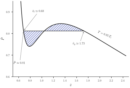
The \(\tilde{T}=0.95\) isotherm is shown in Fig. 9.15. Counting squares permits the equal area construction shown, giving the approximate roots indicated on the figure. Refinement of these roots by the analytic method of Example 2 yields \(\tilde{P}=0.814\), \(\tilde{v}_{g}=1.71\) and \(\tilde{v}_{\ell}=0.683\)
Problem 9.4-8
Using the two points at \(\tilde{T}=0.95\) and \(\tilde{T}=1\) on the coexistence curve of a fluid obeying the van der Waals equation of state (Problem 9.4-7), calculate the average latent heat of vaporization over this range. Specifically apply this result to \(\mathrm{H}_{2} \mathrm{O}\).
Problem 9.4-9
Plot the van der Waals isotherm, in reduced variables, for \(T=0.9 T_{c}\). Make an equal area construction by counting squares on the graph paper. Corroborate and refine this estimate by the method of Example 2.
Problem 9.4-10
Repeat problem 9.4-8 in the range \(0.90 \leq \tilde{T} \leq 0.95\), using the results of problems 9.4-7 and 9.4-9. Does the latent heat vary as the temperature approaches \(T_{c}\) ? What is the expected value of the latent heat precisely at \(T_{c}\) ? The latent heat of vaporization of water at atmospheric pressure is \(\simeq 540\) calories per gram. Is this value qualitatively consistent with the trend suggested by your results?
Problem 9.4-11
Two moles of a van der Waals fluid are maintained at a temperature \(T=0.95 T_{c}\) in a volume of \(200 \mathrm{~cm}^{3}\). Find the mole number and volume of each phase. Use the van der Waals constants of oxygen.
9-5 GENERAL ATTRIBUTES OF FIRST-ORDER PHASE TRANSITIONS
Our discussion of first-order transitions has been based on the general shape of realistic isotherms, of which the van der Waals isotherm is a characteristic representative. The problem can be viewed in a more general perspective based on the convexity or concavity of thermodynamic potentials.
Consider a general thermodynamic potential, \(U\left[P_{s}, \ldots, P_{t}\right]\), that is a function of \(S, X_{1}, X_{2}, \ldots, X_{s-1}, P_{s}, \ldots, P_{t}\). The criterion of stability is that \(U\left[P_{s}, \ldots, P_{t}\right]\) must be a convex function of its extensive parameters and a concave function of its intensive parameters. Geometrically, the function must lie above its tangent hyperplanes in the \(X_{1}, \ldots, X_{s-1}\) subspace and below its tangent hyperplanes in the \(P_{s}, \ldots, P_{t}\) subspace.
Consider the function \(U\left[P_{s}, \ldots, P_{t}\right]\) as a function of \(X_{j}\), and suppose it to have the form shown in Fig. 9.16a. A tangent line \(D O\) is also shown. It will be noted that the function lies above this tangent line. It also lies above all tangent lines drawn at points to the left of \(D\) or to the right of \(O\). The function does not lie above tangent lines drawn to points intermediate between \(D\) and \(O\). The local curvature of the potential is positive for all points except those between points \(F\) and \(M\). Nevertheless a phase
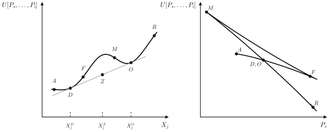
transition occurs from the phase at \(D\) to the phase at \(O\). Global curvature fails (becomes negative) at \(D\) before local curvature fails at \(F\).
The “amended” thermodynamic potential \(U\left[P_{s}, \ldots, P_{t}\right]\) consists of the segment \(A D\) in Fig. 9.15a, the straight line two-phase segment \(D O\), and the original segment \(O R\).
An intermediate point on the straight line segment, such as \(Z\), corresponds to a mixture of phases \(D\) and \(O\). The mole fraction of phase \(D\) varies linearly from unity to zero as \(Z\) moves from point \(D\) to point \(O\), from which it immediately follows that
\[ X=\frac{\left(X_{j}^{0}-X_{j}^{Z}\right)}{\left(X_{j}^{0}-X_{j}^{D}\right)} \]
This is again the “lever rule.” The value of the thermodynamic potential \(U\left[P_{s}, \ldots, P_{t}\right]\) in the mixed state (i.e., at \(Z\) ) clearly is less than that in the pure state (on the initial curve corresponding to \(X_{j}^{z}\) ). Thus the mixed state given by the straight line construction does minimize \(U\left[P_{s}, \ldots, P_{t}\right]\) and does correspond to the physical equilibrium state of the system.
The dependence of \(U\left[P_{s}, \ldots, P_{t}\right]\) on an intensive parameter \(P_{s}\) is subject to similar considerations, which should now appear familiar. The Gibbs potential \(U[T, P]=N \mu(T, P)\) is the particular example studied in the preceding section. The local curvature is negative except for the segment \(M F\) (Fig. 9.16b). But the segment \(M D\) lies above, rather than below, the tangent drawn to the segment \(A D F\) at \(D\). Only the curve \(A D O R\) lies everywhere below the tangent lines, thereby satisfying the conditions of global stability.
Thus the particular results of the preceding section are of very general applicability to all thermodynamic potentials.
PROBLEMS
Problem 9.6-1
In a particular system, solute \(A\) and solute \(B\) are each dissolved in solvent \(C\).
What is the dimensionality of the space in which the phase regions exist?
What is the dimensionality of the region over which two phases coexist?
What is the dimensionality of the region over which three phases coexist?
What is the maximum number of phases that can coexist in this system?
Problem 9.6-2
If \(g\), the molar Gibbs function, is a convex function of \(x_{1}, x_{2}, \ldots, x_{r-1}\), show that a change of variables to \(x_{2}, x_{3}, \ldots, x_{r}\) results in \(g\) being a convex function of \(x_{2}, x_{3}, \ldots, x_{r}\). That is, show that the convexity condition of the molar Gibbs potential is independent of the choice of the “redundant” mole fraction.
Problem 9.6-3
Show that the conditions of stability in a multicomponent system require that the partial molar Gibbs potential \(\mu_{j}\) of any component be an increasing function of the mole fraction \(x_{j}\) of that component, both at constant \(v\) and at constant \(P\), and both at constant \(s\) and at constant \(T\).
PROBLEMS
Problem 9.7-1
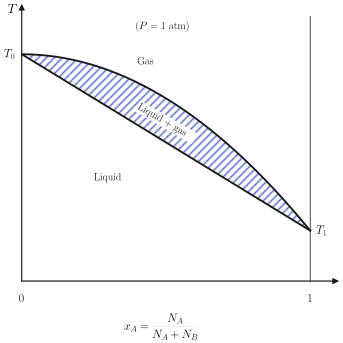
The phase diagram of a solution of \(A\) in \(B\), at a pressure of 1 atm, is as shown. The upper bounding curve of the two-phase region can be represented by
\[ T=T_{0}-\left(T_{0}-T_{1}\right) x_{A}^{2} \]
 The lower bounding curve can be represented by
\[ T=T_{0}-\left(T_{0}-T_{1}\right) x_{A}\left(2-x_{A}\right) \]
A beaker containing equal mole numbers of \(A\) and \(B\) is brought to its boiling temperature. What is the composition of the vapor as it first begins to boil off? Does boiling tend to increase or decrease the mole fraction of \(A\) in the remaining liquid?
Answer:
\[ x_{A}(\text { vapor })=0.866 \]
Problem 9.7-2
Show that if a small fraction \((-d N / N)\) of the material is boiled off the system referred to in Problem 9.7-1, the change in the mole fraction in the remaining liquid is
\[ d x_{A}=-\left[\left(2 x_{A}-x_{A}^{2}\right)^{\frac{1}{2}}-x_{A}\right]\left(\frac{-d N}{N}\right) \]
Problem 9.7-3
The phase diagram of a solution of \(A\) in \(B\), at a pressure of 1 atm and in the region of small mole fraction \(\left(x_{A} \ll 1\right)\), is as shown. The upper bounding
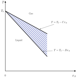 curve of the two-phase region can be represented by
\[ T=T_{0}-C x_{A} \]
and the lower bounding curve by
\[ T=T_{0}-D x_{A} \]
in which \(C\) and \(D\) are positive constants \((D>C)\). Assume that a liquid of mole fraction \(x_{A}^{\circ}\) is brought to a boil and kept boiling until only a fraction \(\left(N_{f} / N_{t}\right)\) of the material remains; derive an expression for the final mole fraction of \(A\).
Show that if \(D=3 C\) and if \(N_{f} / N_{i}=\frac{1}{2}\), the final mole fraction of component \(A\) is one fourth its initial value.