MAXWELL RELATIONS
7-1 THE MAXWELL RELATIONS
In Section 3.6 we observed that quantities such as the isothermal compressibility, the coefficient of thermal expansion, and the molar heat capacities describe properties of physical interest. Each of these is essentially a derivative \((\partial X / \partial Y)_{Z, W \ldots}\) in which the variables are either extensive or intensive thermodynamic parameters. With a wide range of extensive and intensive parameters from which to choose, in general systems, the number of such possible derivatives is immense. But there are relations among such derivatives, so that a relatively small number of them can be considered as independent; all others can be expressed in terms of these few. Needless to say such relationships enormously simplify thermodynamic analyses. Nevertheless the relationships need not be memorized. There is a simple, straightforward procedure for producing the appropriate relationships as needed in the course of a thermodynamic calculation. That procedure is the subject of this chapter.
As an illustration of the existence of such relationships we recall equations 3.70 to 3.71
\[ \frac{\partial^{2} U}{\partial S \partial V}=\frac{\partial^{2} U}{\partial V \partial S} \]
or \({ }^{\text {® }}\)
\[ -\left(\frac{\partial P}{\partial S}\right)_{V, N_{1}, N_{2} \ldots}=\left(\frac{\partial T}{\partial V}\right)_{S, N_{1}, N_{2}} . \]
This relation is the prototype of a whole class of similar equalities known as the Maxwell relations. These relations arise from the equality of the mixed partial derivatives of the fundamental relation expressed in any of the various possible alternative representations.
Given a particular thermodynamic potential, expressed in terms of its \((t+1)\) natural variables, there are \(t(t+1) / 2\) separate pairs of mixed second derivatives. Thus each potential yields \(t(t+1) / 2\) Maxwell relations.
For a single-component simple system the internal energy is a function of three variables \((t=2)\), and the three \([=(2 \cdot 3) / 2]\) pairs of mixed second derivatives are \(\partial^{2} U / \partial S \partial V=\partial^{2} U / \partial V \partial S, \quad \partial^{2} U / \partial S \partial N=\) \(\partial^{2} U / \partial N \partial S\), and \(\partial^{2} U / \partial V \partial N=\partial^{2} U / \partial N \partial V\). The complete set of Maxwell relations for a single-component simple system is given in the following listing, in which the first column states the potential from which the relation derives, the second column states the pair of independent variables with respect to which the mixed partial derivatives are taken, and the last column states the Maxwell relations themselves. A mnemonic diagram to be described in Section 7.2 provides a mental device for recalling relations of this form. In Section 7.3 we present a procedure for utilizing these relations in the solution of thermodynamic problems.
| \(U\) | \(S, V\) | \(\left(\frac{\partial T}{\partial V}\right)_{S, N}=-\left(\frac{\partial P}{\partial S}\right)_{V, N}\) | (7.3) |
|---|---|---|---|
| \(d U=T d S-P d V+\mu d N\) | \(S, N\) | \(\left(\frac{\partial \boldsymbol{T}}{\partial N}\right)_{S . V}=\left(\frac{\partial \mu}{\partial S}\right)_{V, N}\) | (7.4) |
| \(\boldsymbol{V} \boldsymbol{,} \boldsymbol{N}\) | \(-\left(\frac{\partial P}{\partial N}\right)_{S . V}=\left(\frac{\partial \mu}{\partial V}\right)_{S . N}\) | (7.5) | |
| \(U[T] \equiv F\) | T,V | \(\left(\frac{\partial S}{\partial V}\right)_{T, N}=\left(\frac{\partial P}{\partial T}\right)_{V, N}\) | (7.6) |
| \(d F=-S d T-P d V+\mu d N\) | \(T, N\) | \(-\left(\frac{\partial S}{\partial N}\right)_{T, V}=\left(\frac{\partial \mu}{\partial T}\right)_{V, N}\) | (7.7) |
| \(V, N\) | \(-\left(\frac{\partial P}{\partial N}\right)_{T, V}=\left(\frac{\partial \mu}{\partial V}\right)_{T, N}\) | (7.8) | |
| \(U[P] \equiv H\) | \(S, P\) | \(\left(\frac{\partial T}{\partial P}\right)_{S, N}=\left(\frac{\partial V}{\partial S}\right)_{P, N}\) | (7.9) |
| \(d H=T d S+V d P+\mu d N\) | \(S, N\) | \(\left(\frac{\partial T}{\partial N}\right)_{S, P}=\left(\frac{\partial \mu}{\partial S}\right)_{P, N}\) | (7.10) |
| \(P, N\) | \(\left(\frac{\partial V}{\partial N}\right)_{S, P}=\left(\frac{\partial \mu}{\partial P}\right)_{S, N}\) | (7.11) | |
| \(U[\mu]\) | \(S, V\) | \(\left(\frac{\partial T}{\partial V}\right)_{S, \mu}=-\left(\frac{\partial P}{\partial S}\right)_{V, \mu}\) | (7.12) |
| \(d U[\mu]=T d S-P d V-N d \mu\) | \(S, \mu\) | \(\left(\frac{\partial T}{\partial \mu}\right)_{S . V}=-\left(\frac{\partial N}{\partial S}\right)_{V . \mu}\) | (7.13) |
| \(V, \mu\) | \(\left(\frac{\partial P}{\partial \mu}\right)_{S . V}=\left(\frac{\partial N}{\partial V}\right)_{S . \mu}\) | (7.14) |
| \(U[T, P] \equiv G\) | \(T, P\) | \(-\left(\frac{\partial S}{\partial P}\right)_{T, N}=\left(\frac{\partial V}{\partial T}\right)_{P, N}\) | (7.15) |
|---|---|---|---|
| \(d G=-S d T+V d P+\mu d N\) | \(T, N\) | \(-\left(\frac{\partial S}{\partial N}\right)_{T, P}=\left(\frac{\partial \mu}{\partial T}\right)_{P, N}\) | (7.16) |
| \(P, N\) | \(\left(\frac{\partial V}{\partial N}\right)_{T, P}=\left(\frac{\partial \mu}{\partial P}\right)_{T, N}\) | (7.17) | |
| \(U[T, \mu]\) | \(T, V\) | \(\left(\frac{\partial S}{\partial V}\right)_{T . \mu}=\left(\frac{\partial P}{\partial T}\right)_{V . \mu}\) | (7.18) |
| \(\begin{aligned} d U[T, \mu]= & -S d T-P d V \\ & -N d \mu \end{aligned}\) | \(T, \mu\) | \(\left(\frac{\partial S}{\partial \mu}\right)_{T, V}=\left(\frac{\partial N}{\partial T}\right)_{V, \mu}\) | (7.19) |
| \(\boldsymbol{V}, \boldsymbol{\mu}\) | \(\left(\frac{\partial P}{\partial \mu}\right)_{T, V}=\left(\frac{\partial N}{\partial V}\right)_{T, \mu}\) | (7.20) | |
| \(U[P, \mu]\) | \(S, P\) | \(\left(\frac{\partial T}{\partial P}\right)_{S, \mu}=\left(\frac{\partial V}{\partial S}\right)_{P, \mu}\) | (7.21) |
| \(d U[P, \mu]=T d S+V d P+N d \mu\) | \(\boldsymbol{S}, \mu\) | \(\left(\frac{\partial T}{\partial \mu}\right)_{S_{, P}}=-\left(\frac{\partial N}{\partial S}\right)_{P, \mu}\) | (7.22) |
| \(P, \mu\) | \(\left(\frac{\partial V}{\partial \mu}\right)_{S, P}=-\left(\frac{\partial N}{\partial P}\right)_{S, \mu}\) | (7.23) |
7-2 A THERMODYNAMIC MNEMONIC DIAGRAM
A number of the most useful Maxwell relations can be remembered conveniently in terms of a simple mnemonic diagram. \({ }^{1}\) This diagram, given in Fig. 7.1, consists of a square with arrows pointing upward along the two diagonals. The sides are labeled with the four common thermodynamic potentials, \(F, G, H\), and \(U\), in alphabetical order clockwise around the diagram, the Helmholtz potential \(F\) at the top. The two corners at the left are labeled with the extensive parameters \(V\) and \(S\), and the two corners at the right are labeled with the intensive parameters \(T\) and \(P\). (“Valid Facts and Theoretical Understanding Generate Solutions to Hard Problems” suggests the sequence of the labels.)
Each of the four thermodynamic potentials appearing on the square is flanked by its natural independent variables. Thus \(U\) is a natural function of \(V\) and \(S ; F\) is a natural function of \(V\) and \(T\); and \(G\) is a natural function of \(T\) and \(P\). Each of the potentials also depends on the mole numbers, which are not indicated explicitly on the diagram.
[^17]
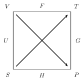
In the differential expression for each of the potentials, in terms of the differentials of its natural (flanking) variables, the associated algebraic sign is indicated by the diagonal arrow. An arrow pointing away from a natural variable implies a positive coefficient, whereas an arrow pointing toward a natural variable implies a negative coefficient. This scheme becomes evident by inspection of the diagram and of each of the following equations:
\[ \begin{aligned} & d U=T d S-P d V+\sum_{k} \mu_{k} d N_{k} \\ & d F=-S d T-P d V+\sum_{k} \mu_{k} d N_{k} \\ & d G=-S d T+V d P+\sum_{k} \mu_{k} d N_{k} \\ & d H=T d S+V d P+\sum_{k} \mu_{k} d N_{k} \end{aligned} \]
Finally the Maxwell relations can be read from the diagram. We then deal only with the corners of the diagram. The labeling of the four corners of the square can easily be seen to be suggestive of the relationship 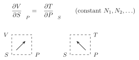 By mentally rotating the square on its side, we find, by exactly the same construction
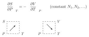
The minus sign in this equation is to be inferred from the unsymmetrical placement of the arrows in this case. The two remaining rotations of the square give the two additional Maxwell relations
\[ \left(\frac{\partial P}{\partial T}\right)_{V}=\left(\frac{\partial S}{\partial V}\right)_{T} \quad\left(\text { constant } N_{1}, N_{2}, \ldots\right) \]
and
\[ \left(\frac{\partial T}{\partial V}\right)_{S}=-\left(\frac{\partial P}{\partial S}\right)_{V} \quad\left(\text { constant } N_{1}, N_{2}, \ldots\right) \]
These are the four most useful Maxwell relations in the conventional applications of thermodynamics.
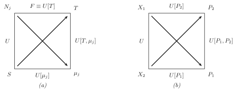
The mnemonic diagram can be adapted to pairs of variables other than \(S\) and \(V\). If we are interested in Legendre transformations dealing with \(S\) and \(N_{f}\), the diagram takes the form shown in Fig. 7.2a. The arrow connecting \(N_{j}\) and \(\mu_{j}\) has been reversed in relation to that which previously connected \(V\) and \(P\) to ake into account the fact that \(\mu_{j}\) is analogous to \(-P\). Equations 7.4, 7.7, 7.13, and 7.19 can be read directly from this diagram. Other diagrams can be constructed in a similar fashion, as indicated in the general case in Fig. 7.2b.
PROBLEMS
Problem 7.2-1
In the immediate vicinity of the state \(T_{0}, v_{0}\) the volume of a particular system of 1 mole is observed to vary according to the relationship
\[ v=v_{0}+a\left(T-T_{0}\right)+b\left(P-P_{0}\right) \]
Calculate the transfer of heat \(d Q\) to the system if the molar volume is changed by a small increment \(d v=v-v_{0}\) at constant temperature \(T_{0}\).
\[ d Q=T\left(\frac{\partial S}{\partial V}\right)_{T} d V=T\left(\frac{\partial P}{\partial T}\right)_{V} d V=-\frac{\begin{array}{c} \text { Answer: } \\ a T \end{array}}{b} d V \]
Problem 7.2-2
For a particular system of 1 mole, in the vicinity of a particular state, a change of pressure \(d P\) at constant \(T\) is observed to be accompanied by a heat flux \(d Q=A d P\). What is the value of the coefficient of thermal expansion of this system, in the same state?
Problem 7.2-3
Show that the relation
\[ \alpha=\frac{1}{T} \]
implies that \(c_{P}\) is independent of the pressure
\[ \left(\frac{\partial \boldsymbol{c}_{\boldsymbol{P}}}{\partial P}\right)_{T}=0 \]
7-3 A PROCEDURE FOR THE REDUCTION OF DERIVATIVES IN SINGLE-COMPONENT SYSTEMS
In the practical applications of thermodynamics the experimental situation to be analyzed frequently dictates a partial derivative to be evaluated. For instance, we may be concerned with the analysis of the temperature change that is required to maintain the volume of a single-component system constant if the pressure is increased slightly. This temperature change is evidently
\[ d T=\left(\frac{\partial T}{\partial P}\right)_{V, N} d P \]
and consequently we are interested in an evaluation of the derivative \((\partial T / \partial P)_{V, N}\). A number of similar problems will be considered in Section 7.4. A general feature of the derivatives that arise in this way is that they are likely to involve constant mole numbers and that they generally involve both intensive and extensive parameters. Of all such derivatives, only three can be independent, and any given derivative can be expressed in terms of an arbitrarily chosen set of three basic derivatives. This set is conventionally chosen as \(c_{P}, \alpha\), and \(\kappa_{T}\).
The choice of \(c_{p}, \alpha\), and \(\kappa_{T}\) is an implicit transformation to the Gibbs representation, for the three second derivatives in this representation are \(\partial^{2} g / \partial T^{2}, \partial^{2} g / \partial T \partial P\), and \(\partial^{2} g / \partial P^{2}\); these derivatives are equal, respectively, to \(-c_{p} / T, v \alpha\), and \(-v \kappa_{T}\). For constant mole numbers these are the only independent second derivatives.
All first derivatives (involving both extensive and intensive parameters) can be written in terms of second derivatives of the Gibbs potential, of which we have now seen that \(c_{p}, \alpha\), and \(\kappa_{T}\) constitute a complete independent set (at constant mole numbers).
The procedure to be followed in this “reduction of derivatives” is straightforward in principle; the entropy \(S\) need only be replaced by \(-\partial G / \partial T\) and \(V\) must be replaced by \(\partial G / \partial P\), thereby expressing the original derivative in terms of second derivatives of \(G\) with respect to \(T\) and \(P\). In practice this procedure can become somewhat involved.
It is essential that the student of thermodynamics become thoroughly proficient in the “reduction of derivatives.” To that purpose we present a procedure, based upon the “mnemonic square” and organized in a step by step recipe that accomplishes the reduction of any given derivative. Students are urged to do enough exercises of this type so that the procedure becomes automatic.
Consider a partial derivative involving constant mole numbers. It is desired to express this derivative in terms of \(c_{P}, \alpha\), and \(\kappa_{T}\). We first recall the following identities which are to be employed in the mathematical manipulations (see Appendix A).
\[ \left(\frac{\partial X}{\partial Y}\right)_{Z}=1 /\left(\frac{\partial Y}{\partial X}\right)_{Z} \]
and
\[ \begin{aligned} & \left(\frac{\partial X}{\partial Y}\right)_{Z}=\left(\frac{\partial X}{\partial W}\right)_{Z} /\left(\frac{\partial Y}{\partial W}\right)_{Z} \\ & \left(\frac{\partial X}{\partial Y}\right)_{Z}=-\left(\frac{\partial Z}{\partial Y}\right)_{X} /\left(\frac{\partial Z}{\partial X}\right)_{Y} \end{aligned} \]
The following steps are then to be taken in order:
- If the derivative contains any potentials, bring them one by one to the numerator and eliminate by the thermodynamic square (equations 7.24 to 7.27).
Example
Reduce the derivative \((\partial P / \partial U)_{G, N}\).
\[ \begin{aligned} \left(\frac{\partial P}{\partial U}\right)_{G, N} & =\left[\left(\frac{\partial U}{\partial P}\right)_{G, N}\right]^{-1} \\ & =\left[T\left(\frac{\partial S}{\partial P}\right)_{G, N}-P\left(\frac{\partial V}{\partial P}\right)_{G, N}\right]^{-1} \\ & =\left[-T\left(\frac{\partial G}{\partial P}\right)_{S, N} /\left(\frac{\partial G}{\partial S}\right)_{P, N}+P\left(\frac{\partial G}{\partial P}\right)_{V, N} /\left(\frac{\partial G}{\partial V}\right)_{P, N}\right]^{-1} \\ & =\left[-T \frac{-S(\partial T / \partial P)_{S, N}+V}{-S(\partial T / \partial S)_{P, N}}+P \frac{-S(\partial T / \partial P)_{V, N}+V}{-S(\partial T / \partial V)_{P, N}}\right]^{-1} \end{aligned} \]
The remaining expression does not contain any potentials but may involve a number of derivatives. Choose these one by one and treat each according to the following procedure. 2. If the derivative contains the chemical potential, bring it to the numerator and eliminate by means of the Gibbs-Duhem relation, \(d \mu=\) \(-s d T+v d P\).
Example
Reduce \((\partial \mu / \partial V)_{S, N}\).
\[ \left(\frac{\partial \mu}{\partial V}\right)_{S, N}=-s\left(\frac{\partial T}{\partial V}\right)_{S, N}+v\left(\frac{\partial P}{\partial V}\right)_{S, N} \]
- If the derivative contains the entropy, bring it to the numerator. If one of the four Maxwell relations of the thermodynamic square now eliminates the entropy, invoke it. If the Maxwell relations do not eliminate the entropy put a \(\partial T\) under \(\partial S\) (employ equation 7.34 with \(w=T\) ). The numerator will then be expressible as one of the specific heats (either \(c_{v}\) or \(c_{P}\) ).
Example
Consider the derivative \((\partial T / \partial P)_{S, N}\) appearing in the example of step 1:
\[ \begin{aligned} \left(\frac{\partial T}{\partial P}\right)_{S, N} & =-\left(\frac{\partial S}{\partial P}\right)_{T, N} /\left(\frac{\partial S}{\partial T}\right)_{P, N} \\ & =\left(\frac{\partial V}{\partial T}\right)_{P, N} / \frac{N}{T} c_{P} \end{aligned} \]
Example
Consider the derivative \((\partial S / \partial V)_{P, N}\). The Maxwell relation would give \((\partial S / \partial V)_{P, N}=(\partial P / \partial T)_{S, N}\) (equation 7.28), which would not eliminate the entropy. We therefore do not invoke the Maxwell relation but write
\[ \left(\frac{\partial S}{\partial V}\right)_{P, N}=\frac{(\partial S / \partial T)_{P, N}}{(\partial V / \partial T)_{P, N}}=\frac{(N / T) c_{P}}{(\partial V / \partial T)_{P, N}} \]
The derivative now contains neither any potential nor the entropy. It consequently contains only \(V, P, T\) (and \(N\) ). 4. Bring the volume to the numerator. The remaining derivative will be expressible in terms of \(\alpha\) and \(\kappa_{T}\).
Example
Given \((\partial T / \partial P)_{V, N}\)
\[ \left(\frac{\partial T}{\partial P}\right)_{V, N}=-\left(\frac{\partial V}{\partial P}\right)_{T, N} /\left(\frac{\partial V}{\partial T}\right)_{P, N}=\frac{\kappa_{T}}{\alpha} \]
- The originally given derivative has now been expressed in terms of the four quantities \(c_{v}, c_{P}, \alpha\), and \(\kappa_{T}\). The specific heat at constant volume is eliminated by the equation
\[ c_{v}=c_{P}-T v \alpha^{2} / \kappa_{T} \]
This useful relation, which should be committed to memory, was alluded to in equation 3.75. The reader should be able to derive it as an exercise (see Problem 7.3-2).
This method of reduction of derivatives can be applied to multicomponent systems as well as to single-component systems, provided that the chemical potentials \(\mu_{j}\) do not appear in the derivative (for the Gibbs-Duhem relation, which eliminates the chemical potential for single-component systems, merely introduces the chemical potentials of other components in multicomponent systems).
PROBLEMS
Problem 7.3-1
Thermodynamicists sometimes refer to the “first \(T d S\) equation” and the “second \(\boldsymbol{T} d \boldsymbol{S}\) equation”;
\[ \begin{array}{ll} T d S=N c_{v} d T+\left(T \alpha / \kappa_{T}\right) d V & (N \text { constant }) \\ T d S=N c_{P} d T-T V \alpha d P & (N \text { constant }) \end{array} \]
Derive these equations.
Problem 7.3-2
Show that the second equation in the preceding problem leads directly to the relation
\[ T\left(\frac{\partial s}{\partial T}\right)_{v}=c_{P}-T v \alpha\left(\frac{\partial P}{\partial T}\right)_{v} \]
and so validates equation 7.36.
Problem 7.3-3
Calculate \((\partial H / \partial V)_{T, N}\) in terms of the standard quantities \(c_{P}, \alpha, \kappa_{T}, T\), and \(P\).
Answer:
\[ \left(\frac{\partial H}{\partial V}\right)_{T, N}=(\boldsymbol{T} \boldsymbol{\alpha}-\mathbf{1}) / \boldsymbol{\kappa}_{T} \]
Problem 7.3-4
Reduce the derivative \((\partial v / \partial s)_{P}\).
Problem 7.3-5
Reduce the derivative \((\partial s / \partial f)_{v}\).
Problem 7.3-6
Reduce the derivative \((\partial s / \partial f)_{P}\).
Problem 7.3-7
Reduce the derivative \((\partial s / \partial v)_{h}\).
7-4 SOME SIMPLE APPLICATIONS
In this section we indicate several representative applications of the manipulations described in Section 7.3. In each case to be considered we first pose a problem. Typically, we are asked to find the change in one parameter when some other parameter is changed. Thus, in the simplest case, we might be asked to find the increase in the pressure of a system if its temperature is increased by \(\Delta T\), its volume being kept constant.
In the examples to be given we consider two types of solutions. First, the straightforward solution that assumes complete knowledge of the fundamental equation, and, second, the solution that can be obtained if \(c_{P}, \alpha\), and \(\kappa_{T}\) are assumed known and if the changes in parameters are small.
Adiabatic Compression
Consider a single-component system of some definite quantity of matter (characterized by the mole number \(N\) ) enclosed within an adiabatic wall. The initial temperature and pressure of the system are known. The system is compressed quasi-statically so that the pressure increases from its initial value \(P_{t}\) to some definite final value \(P_{f}\). We attempt to predict the changes in the various thermodynamic parameters (e.g., in the volume, temperature, internal energy, and chemical potential) of the system.
The essential key to the analysis of the problem is the fact that for a quasi-static process the adiabatic constraint implies constancy of the entropy. This fact follows, of course, from the quasi-static correspondence \(d Q=T d S\).
We consider in particular the change in temperature. First, we assume the fundamental equation to be known. By differentiation, we can find the two equations of state \(T=T(S, V, N)\) and \(P=P(S, V, N)\). By knowing the initial temperature and pressure, we can thereby find the initial volume and entropy. Elimination of \(V\) between the two equations of state gives the temperature as a function of \(S, P\), and \(N\). Then, obviously,
\[ \Delta T=T\left(S, P_{f}, N\right)-T\left(S, P_{i}, N\right) \]
If the fundamental equation is not known, but \(c_{P}, \alpha\), and \(\kappa_{T}\) are given, and if the pressure change is small, we have
\[ d T=\left(\frac{\partial T}{\partial P}\right)_{S, N} d P \]
By the method of Section 7.3, we then obtain
\[ d T=\frac{T v \alpha}{c_{P}} d P \]
The change in chemical potential can be found similarly. Thus, for a small pressure change
\[ \begin{aligned} d \mu & =\left(\frac{\partial \mu}{\partial P}\right)_{S, N} d P \\ & =\left(v-\frac{s T v \alpha}{c_{P}}\right) d P \end{aligned} \]
The fractional change in volume associated with an (infinitesimal) adiabatic compression is characterized by the adiabatic compressibility \(\kappa_{S}\), previously defined in equation 3.73. It was there stated that \(\kappa_{S}\) can be related to \(\kappa_{T}, c_{p}\), and \(\alpha\) (equation 3.76, and (see also Problem 3.9-5), an exercise that is now left to the reader in Problem 7.4-8.
Isothermal Compression
We now consider a system maintained at constant temperature and mole number and quasi-statically compressed from an initial pressure \(P_{t}\) to a final pressure \(P_{f}\). We may be interested in the prediction of the changes in the values of \(U, S, V\), and \(\mu\). By appropriate elimination of variables among the fundamental equation and the equations of state, any such parameter can be expressed in terms of \(T, P\), and \(N\), and the change in that parameter can then be computed directly.
For small changes in pressure we find
\[ \begin{aligned} d S & =\left(\frac{\partial S}{\partial P}\right)_{T, N} d P \\ & =-\alpha V d P \end{aligned} \]
also
\[ \begin{aligned} d U & =\left(\frac{\partial U}{\partial P}\right)_{T, N} d P \\ & =\left(-T \alpha V+P V \kappa_{T}\right) d P \end{aligned} \]
and similar equations exist for the other parameters. One may inquire about the total quantity of heat that must be extracted from the system by the heat reservoir in order to keep the system at constant temperature during the isothermal compression. First, assume that the fundamental equation is known. Then
\[ \Delta Q=T \Delta S=T S\left(T, P_{f}, N\right)-T S\left(T, P_{i}, N\right) \]
where \(S(U, V, N)\) is reexpressed as a function of \(T, P\), and \(N\) in standard fashion.
If the fundamental equation is not known we consider an infinitesimal isothermal compression, for which we have, from equation 7.43
\[ d Q=-T \alpha V d P \]
Finally, suppose that the pressure change is large, but that the fundamental equation is not known (so that the solution 7.46 is not available). Then, if \(\alpha\) and \(V\) are known as functions of \(T\) and \(P\), we integrate equation 7.47 at constant temperature
\[ \Delta Q=-T \int_{P_{i}}^{P_{f}} \alpha V d P \]
This solution must be equivalent to that given in equation 7.46.
Free Expansion
The third process we shall consider is a free expansion (recall Problems 3.4-8 and 4.2-3). The constraints that require the system to have a volume \(V_{i}\) are suddenly relaxed, allowing the system to expand to a volume \(V_{f}\). If the system is a gas (which, of course, does not have to be the case), the expansion may be accomplished conveniently by confining the gas in one section of a rigid container, the other section of which is evacuated. If the septum separating the sections is suddenly fractured the gas spontaneously expands to the volume of the whole container. We seek to predict the change in the temperature and in the various other parameters of the system.
The total internal energy of the system remains constant during the free expansion. Neither heat nor work are transferred to the system by any external agency.
If the temperature is expressed in terms of \(U, V\), and \(N\), we find
\[ T_{f}-T_{i}=T\left(U, V_{f}, N\right)-T\left(U, V_{i}, N\right) \]
If the volume change is small
\[ \begin{aligned} d T & =\left(\frac{\partial T}{\partial V}\right)_{U, N} d V \\ & =\left(\frac{P}{N c_{v}}-\frac{T \alpha}{N c_{v} \kappa_{T}}\right) d V \end{aligned} \]
This process, unlike the two previously treated, is essentially irreversible and is not quasi-static (Problem 4.2-3).
Example
In practice the processes of interest rarely are so neatly defined as those just considered. No single thermodynamic parameter is apt to be constant in the process. More typically, measurements might be made of the temperature during the expansion stroke in the cylinder of an engine. The expansion is neither isothermal nor isentropic, for heat tends to flow uncontrolled through the cylinder walls. Nevertheless, the temperature can be evaluated empirically as a function of the volume, and this defines the process. Various other characterizations of real processes will occur readily to the reader, but the general methodology is well represented by the following particular example. \(N\) moles of a material are expanded from \(V_{1}\) to \(V_{2}\) and the temperature is observed to decrease from \(T_{1}\) to \(T_{2}\), the temperature falling linearly with volume. Calculate the work done on the system and the heat transfer, expressing each result in terms of definite integrals of the tabulated functions \(c_{p}, \alpha\), and \(\kappa_{T}\). Solution We first note that the tabulated functions \(c_{p}(T, P), \alpha(T, P), \kappa_{T}(T, P)\), and \(v(T, P)\) are redundant. The first three functions imply the last, as has already been shown in the example of Section 3.9.
Turning to the stated problem, the equation of the path in the \(T-V\) plane is
\[ T=A+B V ; \quad A=\left(T_{1} V_{2}-T_{2} V_{I}\right) /\left(V_{2}-V_{1}\right) ; \quad B=\left(T_{2}-T_{1}\right) /\left(V_{2}-V_{1}\right) \]
Furthermore, the pressure is known at each point on the path, for the known function \(v(T, P)\) can be inverted to express \(P\) as a function of \(T\) and \(v\), and thence of \(v\) alone
\[ P=P(T, V)=P(A+B V, V) \]
The work done in the process is then
\[ W=\int_{V_{1}}^{V_{2}} P(A+B V, V) d V \]
This integral must be performed numerically, but generally it is well within the capabilities of even a modest programmable hand calculator.
The heat input is calculated by considering \(S\) as a function of \(T\) and \(V\).
\[ \begin{aligned} d S & =\left(\frac{\partial S}{\partial T}\right)_{V} d T+\left(\frac{\partial S}{\partial V}\right)_{T} d V \\ & =\frac{N}{T} c_{v} d T+\left(\frac{\partial P}{\partial T}\right)_{V} d V \\ & =\left(\frac{N c_{p}}{T}-\frac{V \alpha^{2}}{\kappa_{T}}\right) d T+\frac{\alpha}{\kappa_{T}} d V \end{aligned} \]
But on the path, \(d T=B d V\), so that
\[ d S=\left(N B \frac{c_{p}}{T}-\frac{B V \alpha^{2}}{\kappa_{T}}+\frac{\alpha}{\kappa_{T}}\right) d V \]
Thus the heat input is
\[ Q=\int_{V_{1}}^{V_{2}}\left[N B c_{p}-(A+B V)(B V \alpha-1) \alpha / \kappa_{T}\right] d V \]
Again the factors in the integral must be evaluated at the appropriate values of \(P\) and \(T\) corresponding to the point \(V\) on the path, and the integral over \(V\) must then be carried out numerically.
It is often convenient to approximate the given data by polynomial expressions in the region of interest; numerous packaged computer programs for such “fits” are available. Then the integrals can be evaluated either numerically or analytically.
Example
In the \(P-v\) plane of a particular substance, two states, \(A\) and \(D\), are defined by
\[ \begin{array}{ll} P_{A}=10^{5} \mathrm{~Pa} & v_{A}=2 \times 10^{-2} \mathrm{~m}^{3} / \mathrm{mole} \\ P_{D}=10^{4} \mathrm{~Pa} & v_{D}=10^{-1} \mathrm{~m}^{3} / \mathrm{mole} \end{array} \]
and it is also ascertained that \(T_{A}=350.9 \mathrm{~K}\). If 1 mole of this substance is initially in the state \(A\), and if a thermal reservoir at temperature 150 K is available, how much work can be delivered to a reversible work source in a process that leaves the system in the state \(D\) ?
The following data are available. The adiabats of the system are of the form
\[ P v^{2}=\text { constant } \quad(\text { for } s=\text { constant }) \]
Measurements of \(c_{p}\) and \(\alpha\) are known only at the pressure of \(10^{5} \mathrm{~Pa}\).
\[ \begin{array}{ll} c_{p}=B v^{2 / 3} & \left(\text { for } P=10^{5} \mathrm{~Pa}\right) ; \\ & B=10^{8 / 3}=464.2 \mathrm{~J} / \mathrm{m}^{2} \mathrm{~K} \\ \alpha=3 / T & \left(\text { for } P=10^{5} \mathrm{~Pa}\right) \end{array} \]
and no measurements of \(\kappa_{T}\) are available. The reader is strongly urged to analyze this problem independently before reading the following solution.
Solution
In order to assess the maximum work that can be delivered in a reversible process \(A \rightarrow D\) it is necessary only to know \(u_{D}-u_{A}\) and \(s_{D}-s_{A}\).
The adiabat that passes through the state \(D\) is described by \(P v^{2}=10^{2} \mathrm{~Pa} \cdot \mathrm{~m}^{6}\); it intersects the isobar \(P=10^{5} \mathrm{~Pa}\) at a point \(C\) for which
\[ P_{C}=10^{5} \mathrm{~Pa} \quad v_{c}=10^{-3 / 2} \mathrm{~m}^{3}=3.16 \times 10^{-2} \mathrm{~m}^{3} \]
As a two-step quasi-static process joining \(A\) and \(D\) we choose the isobaric process \(A \rightarrow C\) followed by the isentropic process \(C \rightarrow D\). By considering these two processes in turn we seek to evaluate first \(u_{C}-u_{A}\) and \(s_{C}-s_{A}\) and then \(u_{D}-u_{C}\) and \(s_{D}-s_{C}\), yielding finally \(u_{D}-u_{A}\) and \(s_{D}-s_{A}\).
We first consider the isobaric process \(A \rightarrow C\).
\[ d u=T d s-P d v=\left(\frac{c_{p}}{v \alpha}-P\right) d v=\left(\frac{1}{3} B v^{-1 / 3} T-P_{A}\right) d v \]
We cannot integrate this directly for we do not yet know \(T(v)\) along the isobar. To calculate \(T(v)\) we write
\[ \left(\frac{\partial T}{\partial v}\right)_{P}=\frac{1}{v \alpha}=\frac{T}{3 v} \quad\left(\text { for } P=P_{A}\right) \]
or integrating
\[ \ln \left(\frac{T}{T_{A}}\right)=\frac{1}{3} \ln \left(\frac{v}{v_{A}}\right) \]
and
\[ T=350.9 \times(50 v)^{1 / 3} \quad\left(\text { on } P=10^{5} \mathrm{~Pa} \text { isobar }\right) \]
Returning now to the calculation of \(u_{C}-u_{A}\)
\[ d u=\left[\frac{1}{3} B \times 350.9 \times(50)^{1 / 3}-10^{5}\right] d v \approx 10^{5} d v \]
or
\[ u_{C}-u_{A}=10^{5} \times\left(v_{C}-v_{A}\right)=1.16 \times 10^{3} \mathrm{~J} \]
We now require the difference \(u_{D}-u_{C}\). Along the adiabat we have
\[ u_{D}-u_{C}=-\int_{v_{C}}^{v_{D}} P d v=-10^{2} \int_{v_{C}}^{v_{D}} \frac{d v}{v^{2}}=10^{2}\left[v_{D}^{-1}-v_{C}^{-1}\right]=-2.16 \times 10^{3} \mathrm{~J} \]
Finally, then, we have the required energy difference
\[ u_{D}-u_{A}=-10^{3} \mathrm{~J} \]
We now turn our attention to the entropy difference \(s_{D}-s_{A}-s_{C}-s_{A}\). Along the isobar \(A C\)
\[ d s=\left(\frac{\partial s}{\partial v}\right)_{P} d v=\frac{c_{P}}{T v \alpha} d v=\frac{1}{3} B v^{-1 / 3} d v \]
and
\[ s_{D}-s_{A}=s_{C}-s_{A}=\frac{1}{2} B\left[v_{C}^{2 / 3}-v_{A}^{2 / 3}\right]=6.1 \mathrm{~J} / \mathrm{K} \]
Knowing \(\Delta u\) and \(\Delta s\) for the process, we turn to the problem of delivering maximum work. The increase in entropy of the system permits us to extract energy from the thermal reservoir.
\[ \left(-Q_{\mathrm{res}}\right)=T_{\mathrm{res}} \Delta s=150 \times 6.1=916 \mathrm{~J} \]
The total energy that can then be delivered to the reversible work source is ( \(-\Delta u)+\left(-Q_{\text {res }}\right.\) ), or
\[ \text { work delivered }=1.92 \times 10^{3} \mathbf{J} \]
PROBLEMS
Problem 7.4-1
In the analysis of a Joule-Thomson experiment we may be given the initial and final molar volumes of the gas, rather than the initial and final pressures. Express the derivative \((\partial T / \partial v)_{h}\) in terms of \(c_{p}, \alpha\), and \(\kappa_{T}\).
Problem 7.4-2
The adiabatic bulk modulus is defined by
\[ \beta_{S}=-v\left(\frac{\partial P}{\partial v}\right)_{s}=-V\left(\frac{\partial P}{\partial V}\right)_{S, N} \]
Express this quantity in terms of \(c_{p}, c_{v}, \alpha\), and \(\kappa_{T}\) (do not eliminate \(c_{p}\) ). What is the relation of your result to the identity \(\kappa_{s} / \kappa_{T}=c_{v} / c_{p}\) (recall Problem 3.9-5)?
Problem 7.4-3
Evaluate the change in temperature in an infinitesimal free expansion of a simple ideal gas (equation 7.51). Does this result also hold if the change in volume is comparable to the initial volume? Can you give a more general argument for a simple ideal gas, not based on equation 7.51?
Problem 7.4-4
Show that equation 7.46 can be written as
\[ Q=U_{f}[P, \mu]-U_{i}[P, \mu] \]
so that \(U[P, \mu]\) can be interpreted as a “potential for heat at constant \(T\) and \(N\).”
Problem 7.4-5
A 1% decrease in volume of a system is carried out adiabatically. Find the change in the chemical potential in terms of \(c_{p}, \alpha\), and \(\kappa_{T}\) (and the state functions \(P, T, u, v, s\), etc).
Problem 7.4-6
Two moles of an imperfect gas occupy a volume of 1 liter and are at a temperature of 100 K and a pressure of 2 MPa . The gas is allowed to expand freely into an additional volume, initially evacuated, of \(10 \mathrm{~cm}^{3}\). Find the change in enthalpy.
At the initial conditions \(c_{p}=0.8 \mathrm{~J} /\) mole \(\cdot \mathrm{K}, \kappa_{T}=3 \times 10^{6} \mathrm{~Pa}^{-1}\), and \(\alpha=\) \(0.002 \mathrm{~K}^{-1}\).
Answer:
\[ \Delta H=\left[\frac{P-\left(c_{p}-P v \alpha\right)}{\left(c_{p} \kappa_{T}-T v \alpha^{2}\right)}\right] \Delta v=15 \mathrm{~J} \]
Problem 7.4-7
Show that \(\left(\partial c_{v} / \partial v\right)_{T}=T\left(\partial^{2} P / \partial T^{2}\right)_{v}\) and evaluate this quantity for a system obeying the van der Waals equation of state.
Problem 7.4-8
Show that
\[ \left(\frac{\partial c_{p}}{\partial P}\right)_{T}=-T v\left[\alpha^{2}+\left(\frac{\partial \alpha}{\partial T}\right)_{P}\right] \]
Evaluate this quantity for a system obeying the equation of state
\[ P\left(v+\frac{A}{T^{2}}\right)=R T \]
Problem 7.4-9
One mole of the system of Problem 7.4-8 is expanded isothermally from an initial pressure \(P_{0}\) to a final pressure \(P_{f}\). Calculate the heat flux to the system in this process.
Answer:
\[ Q=-R T \ln \left(\frac{P_{f}}{P_{t}}\right)-2 A\left(P_{f}-P_{t}\right) / T^{2} \]
Problem 7.4-10
A system obeys the van der Waals equation of state. One mole of this system is expanded isothermally at temperature \(T\) from an initial volume \(v_{0}\) to a final volume \(v_{f}\). Find the heat transfer to the system in this expansion.
Problem 7.4-11
Two moles of \(\mathrm{O}_{2}\) are initially at a pressure of \(10^{5} \mathrm{~Pa}\) and a temperature of \(0^{\circ} \mathrm{C}\). An adiabatic compression is carried out to a final temperature of \(300^{\circ} \mathrm{C}\). Find the final pressure by integration of equation 7.39. Assume that \(\mathrm{O}_{2}\) is a simple ideal gas with a molar heat capacity \(c_{p}\) which can be represented by
\[ c_{p}=26.20+11.49 \times 10^{-3} T-3.223 \times 10^{-6} T^{2} \]
where \(c_{p}\) is in \(\mathrm{J} /\) mole and \(T\) is in kelvins. Answer:
\[ P_{f} \simeq 15 \times 10^{5} \mathrm{~Pa} \]
Problem 7.4-12
A ball bearing of mass 10 g just fits in a vertical glass tube of cross-sectional area \(2 \mathrm{~cm}^{2}\). The bottom of the tube is connected to a vessel of volume 5 liters, filled with oxygen at a temperature of \(30^{\circ} \mathrm{C}\). The top of the tube is open to the atmosphere, which is at a pressure of \(10^{5} \mathrm{~Pa}\) and a temperature of \(30^{\circ} \mathrm{C}\). What is the period of vertical oscillation of the ball? Assume that the compressions and expansions of the oxygen are slow enough to be essentially quasi-static but fast enough to be adiabatic. Assume that \(\mathrm{O}_{2}\) is a simple ideal gas with a molar heat capacity as given in Problem 7.4-11.
Problem 7.4-13
Calculate the change in the molar internal energy in a throttling process in which the pressure change is \(d P\), expressing the result in terms of standard parameters.
Problem 7.4-14
Assuming that a gas undergoes a free expansion and that the temperature is found to change by \(d T\), calculate the difference \(d P\) between the initial and final pressure.
Problem 7.4-15
One mole of an ideal van der Waals fluid is contained in a vessel of volume \(V_{i}\) at temperature \(T_{i}\). A valve is opened, permitting the fluid to expand into an initially evacuated vessel, so that the final volume is \(V_{f}\). The walls of the vessels are adiabatic. Find the final temperature \(T_{f}\).
Evaluate your result for \(V_{t}=2 \times 10^{-3} \mathrm{~m}^{3}, V_{f}=5 \times 10^{-3} \mathrm{~m}^{3}, N=1, T_{t}=300\) K, and the van der Waals constants are those of argon (Table 3.1). What was the initial pressure of the gas?
Problem 7.4-16
Assuming the expansion of the ideal van der Waals fluid of Problem 7.4-15 to be carried out quasi-statically and adiabatically, again find the final temperature \(T_{f}\).
Evaluate your result with the numerical data specified in Problem 7.4-15.
Problem 7.4-17
It is observed that an adiabatic decrease in molar volume of 1% produces a particular change in the chemical potential \(\mu\). What percentage change in molar volume, carried out isothermally, produces the same change in \(\mu\) ?
Problem 7.4-18
A cylinder is fitted with a piston, and the cylinder contains helium gas. The sides of the cylinder are adiabatic, impermeable, and rigid, but the bottom of the cylinder is thermally conductive, permeable to helium, and rigid. Through this permeable wall the system is in contact with a reservoir of constant \(T\) and \(\mu_{\mathrm{He}}\) (the chemical potential of He). Calculate the compressibility of the system \([-(1 / V)(d V / d P)]\) in terms of the properties of helium \(\left(c_{p}, v, \alpha, \kappa_{T}\right.\), etc.) and thereby demonstrate that this compressibility diverges. Discuss the physical reason for this divergence.
Problem 7.4-19
The cylinder in Problem 7.4-18 is initially filled with \(\frac{1}{10}\) mole of Ne. Assume both He and Ne to be monatomic ideal gases. The bottom of the cylinder is again permeable to He, but not to Ne. Calculate the pressure in the cylinder and the compressibility \((-1 / V)(d V / d P)\) as functions of \(T, V\), and \(\mu_{\mathrm{He}}\).
Hint: Recall Problems 5.3-1, 5.3-10, and 6.2-3.
Problem 7.4-20
A system is composed of 1 mole of a particular substance. In the \(P-v\) plane two states ( \(A\) and \(B\) ) lie on the locus \(P v^{2}=\) constant, so that \(P_{A} v_{A}^{2}=P_{B} v_{B}^{2}\). The following properties of the system have been measured along this locus: \(c_{p}=C v^{2}, \alpha=D / v\), and \(\kappa_{T}=E v\), where \(C, D\), and \(E\) are constants. Calculate the temperature \(T_{B}\) in terms of \(T_{A}, P_{A}, v_{A}, v_{B}\), and the constants \(C, D\), and \(E\).
Answer:
\[ T_{B}=T_{A}+\left(v_{B}-v_{A}\right) / D+2 E P_{A} v_{A}^{2} D^{-1} \ln \left(v_{B} / v_{a}\right) \]
Problem 7.4-21
A system is composed of 1 mole of a particular substance. Two thermodynamic states, designated as \(A\) and \(B\), lie on the locus \(P v=\) constant . The following properties of the system have been measured along this locus; \(c_{p}=C v\), \(\alpha=D / v^{2}\), and \(\kappa_{T}=E v\), where \(C, D\), and \(E\) are constants. Calculate the difference in molar energies ( \(u_{B}-u_{A}\) ) in terms of \(T_{A}, P_{A}, v_{A}, v_{B}\), and the constants \(C, D\), and \(E\).
Problem 7.4-22
The constant-volume heat capacity of a particular simple system is
\[ c_{v}=A T^{3} \quad(A=\text { constant }) \]
In addition the equation of state is known to be of the form
\[ \left(v-v_{0}\right) P=B(T) \]
where \(B(T)\) is an unspecified function of \(T\). Evaluate the permissible functional form of \(B(T)\).
In terms of the undetermined constants appearing in your functional representation of \(B(T)\), evaluate \(\alpha, c_{p}\), and \(\kappa_{T}\) as functions of \(T\) and \(v\). Hint: Examine the derivative \(\partial^{2} s / \partial T \partial v\). Answer:
\[ c_{p}=A T^{3}+\left(T^{3} / D T+E\right) \text {, where } D \text { and } E \text { are constants. } \]
Problem 7.4-23
A system is expanded along a straight line in the \(P-v\) plane, from the initial state \(\left(P_{0}, v_{0}\right)\) to the final state \(\left(P_{f}, v_{f}\right)\). Calculate the heat transfer per mole to the system in this process. It is to be assumed that \(\alpha, \kappa_{T}\), and \(c_{p}\) are known only along the isochore \(v=v_{0}\) and the isobar \(P=P_{f}\); in fact it is sufficient to specify that the quantity \(\left(c_{v} \kappa_{T} / \alpha\right)\) has the value \(A P\) on the isochore \(v=v_{0}\), and the quantity ( \(c_{p} / v \alpha\) ) has the value \(B v\) on the isobar \(P=P_{f}\), where \(A\) and \(B\) are known constants. That is
\[ \begin{array}{ll} \frac{c_{v} \kappa_{T}}{\alpha}=A P & \left(\text { for } v=v_{0}\right) \\ \frac{c_{p}}{v \alpha}=B v & \left(\text { for } P=P_{f}\right) \end{array} \]
Answer:
\[ Q=\frac{1}{2} A\left(P_{f}^{2}-P_{0}^{2}\right)+\frac{1}{2} B\left(v_{f}^{2}-v_{0}^{2}\right)+\frac{1}{2}\left(P_{0}-P_{f}\right)\left(v_{f}-v_{0}\right) \]
Problem 7.4-24
A nonideal gas undergoes a throttling process (i.e., a Joule-Thomson expansion) from an initial pressure \(P_{0}\) to a final pressure \(P_{f}\). The initial temperature is \(T_{0}\) and the initial molar volume is \(v_{0}\). Calculate the final temperature \(T_{f}\) if it is given that
\[ \begin{aligned} \kappa_{T} & =\frac{A}{v^{2}} \text { along the } T=T_{0} \text { isotherm }(A>0) \\ \alpha & =\alpha_{0} \text { along the } T=T_{0} \text { isotherm } \end{aligned} \]
and
\[ c_{p}=c_{p}^{0} \text { along the } P=P_{f} \text { isobar } \]
What is the condition on \(T_{0}\) in order that the temperature be lowered by the expansion?
7-5 GENERALIZATIONS: MAGNETIC SYSTEMS
For systems other than simple systems there exists a complete parallelism to the formalism of Legendre transformation, of Maxwell relations, and of reduction of derivatives by the mnemonic square.
The fundamental equation of a magnetic system is of the form (recall Section 3.8 and Appendix B)
\[ U=U(S, V, I, N) \]
Legendre transformations with respect to \(S, V\), and \(N\) simply retain the magnetic moment \(I\) as a parameter. Thus the enthalpy is a function of \(S\), \(P, I\), and \(N\).
\[ H \equiv U[P]=U+P V=H(S, P, I, N) \]
An analogous transformation can be made with respect to the magnetic coordinate
\[ U\left[B_{e}\right]=U-B_{e} I \]
and this potential is a function of \(S, V, B_{e}\), and \(N\). The condition of equilibrium for a system at constant external field is that this potential be minimum.
Various other potentials result from multiple Legendre transformations, as depicted in the mnemonic squares of Fig. 7.3. Maxwell relations and the relationships between potentials can be read from these squares in a completely straightforward fashion.
\[ \begin{aligned} \left(\frac{\partial V}{\partial I}\right)_{S, P} & =\left(\frac{\partial B_{e}}{\partial P}\right)_{S, I} \\ \left(\frac{\partial I}{\partial P}\right)_{S, B_{e}} & =-\left(\frac{\partial V}{\partial B_{e}}\right)_{S, P} \end{aligned} \]
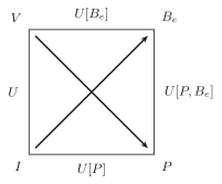
\[ \begin{aligned} \left(\frac{\partial V}{\partial I}\right)_{T, P} & =\left(\frac{\partial B_{e}}{\partial P}\right)_{T, I} \\ \left(\frac{\partial I}{\partial P}\right)_{T, B_{e}} & =-\left(\frac{\partial V}{\partial B_{e}}\right)_{T, P} \end{aligned} \]
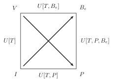
\[ \begin{aligned} & \left(\frac{\partial S}{\partial I}\right)_{V, T}=-\left(\frac{\partial B_{e}}{\partial T}\right)_{V, I} \\ & \left(\frac{\partial T}{\partial I}\right)_{V, S}=\left(\frac{\partial B_{e}}{\partial S}\right)_{V, I} \end{aligned} \]
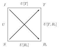
The “magnetic enthalpy” \(U\left[P, B_{e}\right] \equiv U+P V-B_{e} I\) is an interesting and useful potential. It is minimum for systems maintained at constant pressure and constant external field. Furthermore, as in equation 6.29 for the enthalpy, \(d U\left[P, B_{e}\right]=T d S=d Q\) at constant \(P, B_{e}\), and \(N\). Thus the magnetic enthalpy \(U\left[P, B_{e}\right]\) acts as a “potential for heat” for systems maintained at constant pressure and magnetic field.
Example
A particular material obeys the fundamental equation of the “paramagnetic model” (equation 3.66), with \(T_{0}=200 \mathrm{~K}\) and \(\mathrm{I}_{0}^{2} / 2 \mathrm{R}=10 \mathrm{Tesla}^{2} \mathrm{~K} / \mathrm{m}^{2} \mathrm{~J}\). Two moles of this material are maintained at constant pressure in an external field of \(B_{e}=0.2\) Tesla (or 2000 gauss), and the system is heated from an initial temperature of 5 K to a final temperature of 10 K. What is the heat input to the system?
Solution
The heat input is the change in the “magnetic enthalpy” \(U\left[P, B_{e}\right]\). For a system in which the fundamental relation is independent of volume, \(P \equiv \partial U / \partial V=0\), so that \(U\left[P, B_{e}\right]\) degenerates to \(U-B_{e} I=U\left[B_{e}\right]\). Furthermore for the paramagnetic model (equation 3.66), \(U=N R T\) and \(I=\left(N I_{0}^{2} / 2 R T\right) B_{e}\), so that \(U\left[P, B_{e}\right]=U\left[B_{e}\right]=N R T-\left(N I_{0}^{2} / 2 R T\right) B_{e}^{2}\). Thus
\[ \begin{aligned} Q & =N\left[R \Delta T-\frac{I_{0}^{2}}{2 R} B_{e}^{2} \Delta\left(\frac{1}{T}\right)\right] \\ & =2[8314 \times 5+10 \times 0.04 \times 0.1] \mathrm{J}=83.15 \mathrm{~J} \end{aligned} \]
(Note that the magnetic contribution, arising from the second term, is small compared to the nonmagnetic first-term contribution; in reality the nonmagnetic contribution to the heat capacity of real solids falls rapidly at low temperatures and would be comparably small. Recall Problem 3.9-6.)
PROBLEMS
Problem 7.5-1
Calculate the “magnetic Gibbs potential” \(U\left[T, B_{e}\right]\) for the paramagnetic model of equation 3.66. Corroborate that the derivative of this potential with respect to \(B_{e}\) at constant \(T\) has its proper value.
Problem 7.5-2
Repeat Problem 7.5-1 for the system with the fundamental equation given in Problem 3.8-2.
Answer:
\[ U\left[T, B_{e}\right]=\frac{1}{2} N \frac{\chi}{\mu_{0}} B_{e}^{2}-\frac{1}{2} N R T \ln \left(k_{B} T / 2 \varepsilon\right) \]
Problem 7.5-3
Calculate \((\partial I / \partial T)_{s}\) for the paramagnetic model of equation 3.66. Also calculate \(\left(\partial S / \partial B_{e}\right)_{I}\). What is the relationship between these derivatives, as read from the mnemonic square?
Problem 7.5-4
Show that
\[ C_{B_{e}}-C_{I}=\frac{\mu_{0}^{2} T}{\chi_{T}^{2}}\left(\frac{\partial I}{\partial T}\right)_{B_{e}} \]
and
\[ \frac{C_{B_{e}}}{C_{I}}=\frac{\chi_{T}}{\chi_{S}} \]
where \(C_{B_{s}}\) and \(C_{I}\) are heat capacities and \(\chi_{T}\) and \(\chi_{s}\) are susceptibilities: \(\chi_{T} \equiv \mu_{0}\left(\partial I / \partial B_{e}\right)_{T}\).