ALTERNATIVE FORMULATIONS AND LEGENDRE TRANSFORMATIONS
5-1 THE ENERGY MINIMUM PRINCIPLE
In the preceding chapters we have inferred some of the most evident and immediate consequences of the principle of maximum entropy. Further consequences will lead to a wide range of other useful and fundamental results. But to facilitate those developments it proves to be useful now to reconsider the formal aspects of the theory and to note that the same content can be reformulated in several equivalent mathematical forms. Each of these alternative formulations is particularly convenient in particular types of problems, and the art of thermodynamic calculations lies largely in the selection of the particular theoretical formulation that most incisively “fits” the given problem. In the appropriate formulation thermodynamic problems tend to be remarkably simple; the converse is that they tend to be remarkably complicated in an inappropriate formalism!
Multiple equivalent formulations also appear in mechanics-Newtonian, Lagrangian, and Hamiltonian formalisms are tautologically equivalent. Again certain problems are much more tractable in a Lagrangian formalism than in a Newtonian formalism, or vice versa. But the difference in convenience of different formalisms is enormously greater in thermodynamics. It is for this reason that the general theory of transformation among equivalent representations is here incorporated as a fundamental aspect of thermostatistical theory.
In fact we have already considered two equivalent representations-the energy representation and the entropy representation. But the basic extremum principle has been formulated only in the entropy representation. If these two representations are to play parallel roles in the theory we must find an extremum principle in the energy representation, analogous to the entropy maximum principle. There is, indeed, such an extremum principle; the principle of maximum entropy is equivalent to, and can be
replaced by, a principle of minimum energy. Whereas the entropy maximum principle characterizes the equilibrium state as having maximum entropy for given total energy, the energy minimum principle characterizes the equilibrium state as having minimum energy for given total entropy.
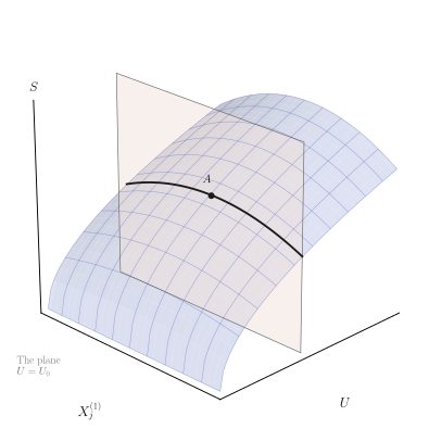
Figure 5.1 shows a section of the thermodynamic configuration space for a composite system, as discussed in Section 4.1. The axes labeled \(S\) and \(U\) correspond to the total entropy and energy of the composite system, and the axis labeled \(X_{j}^{(1)}\) corresponds to a particular extensive parameter of the first subsystem. Other axes, not shown explicitly in the figure, are \(U^{(1)}, X_{j}\), and other pairs \(X_{k}^{(1)}, X_{k}\).
The total energy of the composite system is a constant determined by the closure condition. The geometrical representation of this closure condition is the requirement that the state of the system lie on the plane \(U=U_{0}\) in Fig. 5.1. The fundamental equation of the system is represented by the surface shown, and the representative point of the system therefore must be on the curve of intersection of the plane and the surface. If the parameter \(X_{j}^{(1)}\) is unconstrained, the equilibrium state is the particular state that maximizes the entropy along the permitted curve; the state labeled \(A\) in Fig. 5.1.
The alternative representation of the equilibrium state \(A\) as a state of minimum energy for given entropy is illustrated in Fig. 5.2. Through the
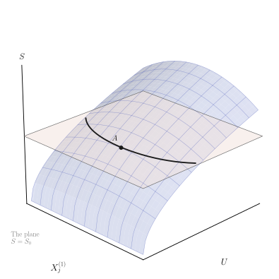
equilibrium point \(A\) is passed the plane \(S=S_{0}\), which determines a curve of intersection with the fundamental surface. This curve consists of a family of states of constant entropy, and the equilibrium state \(A\) is the state that minimizes the energy along this curve.
The equivalence of the entropy maximum and the energy minimum principles clearly depends upon the fact that the geometrical form of the fundamental surface is generally as shown in Fig. 5.1 and 5.2. As discussed in Section 4.1, the form of the surface shown in the figures is determined by the postulates that \(\partial S / \partial U>0\) and that \(U\) is a single-valued continuous function of \(S\); these analytic postulates accordingly are the underlying conditions for the equivalence of the two principles.
To recapitulate, we have made plausible, though we have not yet proved, that the following two principles are equivalent:
Entropy Maximum Principle. The equilibrium value of any unconstrained internal parameter is such as to maximize the entropy for the given value of the total internal energy.
Energy Minimum Principle. The equilibrium value of any unconstrained internal parameter is such as to minimize the energy for the given value of the total entropy.
The proof of the equivalence of the two extremum criteria can be formulated either as a physical argument or as a mathematical exercise. We turn first to the physical argument, to demonstrate that if the energy were not minimum the entropy could not be maximum in equilibrium, and inversely.
Assume, then, that the system is in equilibrium but that the energy does not have its smallest possible value consistent with the given entropy. We could then withdraw energy from the system (in the form of work) maintaining the entropy constant, and we could thereafter return this energy to the system in the form of heat. The entropy of the system would increase \((d Q=T d S)\), and the system would be restored to its original energy but with an increased entropy. This is inconsistent with the principle that the initial equilibrium state is the state of maximum entropy! Hence we are forced to conclude that the original equilibrium state must have had minimum energy consistent with the prescribed entropy.
The inverse argument, that minimum energy implies maximum entropy, is similarly constructed (see Problem 5.1-1).
In a more formal demonstration we assume the entropy maximum principle
\[ \left(\frac{\partial S}{\partial X}\right)_{U}=0 \quad \text { and } \quad\left(\frac{\partial^{2} S}{\partial X^{2}}\right)_{U}<0 \]
where, for clarity, we have written \(X\) for \(X_{j}^{(1)}\), and where it is implicit that all other \(X\) ’s are held constant throughout. Also, for clarity, we temporarily denote the first derivative \((\partial U / \partial X)_{S}\) by \(P\). Then (by equation A. 22 of Appendix A)
\[ P \equiv\left(\frac{\partial U}{\partial X}\right)_{S}=-\frac{\left(\frac{\partial S}{\partial X}\right)_{U}}{\left(\frac{\partial S}{\partial U}\right)_{X}}=-T\left(\frac{\partial S}{\partial X}\right)_{U}=0 \]
We conclude that \(U\) has an extremum. To classify that extremum as a maximum, a minimum, or a point of inflection we must study the sign of the second derivative \(\left(\partial^{2} U / \partial X^{2}\right)_{S} \equiv(\partial P / \partial X)_{S}\). But considering \(P\) as a function of \(U\) and \(X\) we have
\[ \begin{aligned} \left(\frac{\partial^{2} U}{\partial X^{2}}\right)_{S} & =\left(\frac{\partial P}{\partial X}\right)_{S}=\left(\frac{\partial P}{\partial U}\right)_{X}\left(\frac{\partial U}{\partial X}\right)_{S}+\left(\frac{\partial P}{\partial X}\right)_{U}=\left(\frac{\partial P}{\partial U}\right)_{X} P+\left(\frac{\partial P}{\partial X}\right)_{U} \\ & =\left(\frac{\partial P}{\partial X}\right)_{U} \quad \text { at } P=0 \end{aligned} \]
\[ \begin{aligned} & =\frac{\partial}{\partial X}\left[-\frac{\left(\frac{\partial S}{\partial X}\right)_{U}}{\left(\frac{\partial S}{\partial U}\right)_{X}}\right]_{U} \\ & =-\frac{\frac{\partial^{2} S}{\partial X^{2}}}{\frac{\partial S}{\partial U}}+\frac{\partial S}{\partial X} \frac{\frac{\partial^{2} S}{\partial X \partial U}}{\left(\frac{\partial S}{\partial U}\right)^{2}} \\ & =-T \frac{\partial^{2} S}{\partial X^{2}}>0 \quad \text { at } \frac{\partial S}{\partial X}=0 \end{aligned} \]
so that \(U\) is a minimum. The inverse argument is identical in form. As already indicated, the fact that precisely the same situation is described by the two extremal criteria is analogous to the isoperimetric problem in geometry. Thus a circle may be characterized either as the two dimensional figure of maximum area for given perimeter or, alternatively, as the two dimensional figure of minimum perimeter for given area.
The two alternative extremal criteria that characterize a circle are completely equivalent, and each applies to every circle. Yet they suggest two different ways of generating a circle. Suppose we are given a square and we wish to distort it continuously to generate a circle. We may keep its area constant and allow its bounding curve to contract as if it were a rubber band. We thereby generate a circle as the figure of minimum perimeter for the given area. Alternatively we might keep the perimeter of the given square constant and allow the area to increase, thereby obtaining a (different) circle, as the figure of maximum area for the given perimeter. However, after each of these circles is obtained each satisfies both extremal conditions for its final values of area and perimeter.
The physical situation pertaining to a thermodynamic system is very closely analogous to the geometrical situation described. Again, any equilibrium state can be characterized either as a state of maximum entropy for given energy or as a state of minimum energy for given entropy. But these two criteria nevertheless suggest two different ways of attaining equilibrium. As a specific illustration of these two approaches to equilibrium, consider a piston originally fixed at some point in a closed cylinder. We are interested in bringing the system to equilibrium without the constraint on the position of the piston. We can simply remove the constraint and allow the equilibrium to establish itself spontaneously; the entropy increases and the energy is maintained constant by the closure condition. This is the process suggested by the entropy maximum principle. Alternatively, we can permit the piston to move very slowly, reversi- bly doing work on an external agent until it has moved to the position that equalizes the pressure on the two sides. During this process energy is withdrawn from the system, but its entropy remains constant (the process is reversible and no heat flows). This is the process suggested by the energy minimum principle. The vital fact we wish to stress, however, is that independent of whether the equilibrium is brought about by either of these two processes, or by any other process, the final equilibrium state in each case satisfies both extremal conditions.
Finally, we illustrate the energy minimum principle by using it in place of the entropy maximum principle to solve the problem of thermal equilibrium, as treated in Section 2.4. We consider a closed composite system with an internal wall that is rigid, impermeable, and diathermal. Heat is free to flow between the two subsystems, and we wish to find the equilibrium state. The fundamental equation in the energy representation is
\[ U=U^{(1)}\left(S^{(1)}, V^{(1)}, N_{1}^{(1)}, \ldots\right)+U^{(2)}\left(S^{(2)}, V^{(2)}, N_{1}^{(2)}, \ldots\right) \]
All volume and mole number parameters are constant and known. The variables that must be computed are \(S^{(1)}\) and \(S^{(2)}\). Now, despite the fact that the system is actually closed and that the total energy is fixed, the equilibrium state can be characterized as the state that would minimize the energy if energy changes were permitted. The virtual change in total energy associated with virtual heat fluxes in the two systems is
\[ d U=T^{(1)} d S^{(1)}+T^{(2)} d S^{(2)} \]
The energy minimum condition states that \(d U=0\), subject to the condition of fixed total entropy:
\[ S^{(1)}+S^{(2)}=\text { constant } \]
whence
\[ d U=\left(T^{(1)}-T^{(2)}\right) d S^{(1)}=0 \]
and we conclude that
\[ T^{(1)}=T^{(2)} \]
The energy minimum principle thus provides us with the same condition of thermal equilibrium as we previously found by using the entropy maximum principle.
Equation 5.12 is one equation in \(S^{(1)}\) and \(S^{(2)}\). The second equation is most conveniently taken as equation 5.8, in which the total energy \(U\) is known and which consequently involves only the two unknown quantities \(S^{(1)}\) and \(S^{(2)}\). Equations 5.8 and 5.12, in principle, permit a fully explicit solution of the problem.
In a precisely analogous fashion the equilibrium condition for a closed composite system with an internal moveable adiabatic wall is found to be equality of the pressure. This conclusion is straightforward in the energy representation but, as was observed in the last paragraph of Section 2.7, it is relatively delicate in the entropy representation.
PROBLEMS
Problem 5.1-1
Formulate a proof that the energy minimum principle implies the entropy maximum principle-the “inverse argument” referred to after equation 5.7. That is, show that if the entropy were not maximum at constant energy then the energy could not be minimum at constant entropy.
Hint: First show that the permissible increase in entropy in the system can be exploited to extract heat from a reversible heat source (initially at the same temperature as the system) and to deposit it in a reversible work source. The reversible heat source is thereby cooled. Continue the argument.
Problem 5.1-2
An adiabatic, impermeable and fixed piston separates a cylinder into two chambers of volumes \(V_{0} / 4\) and \(3 V_{0} / 4\). Each chamber contains 1 mole of a monatomic ideal gas. The temperatures are \(T_{s}\) and \(T_{l}\), the subscripts \(s\) and \(l\) referring to the small and large chambers, respectively.
The piston is made thermally conductive and moveable, and the system relaxes to a new equilibrium state, maximizing its entropy while conserving its total energy. Find this new equilibrium state.
Consider a small virtual change in the energy of the system, maintaining the entropy at the value attained in part (a). To accomplish this physically we can reimpose the adiabatic constraint and quasistatically displace the piston by imposition of an external force. Show that the external source of this force must do work on the system in order to displace the piston in either direction. Hence the state attained in part (a) is a state of minimum energy at constant entropy.
Reconsider the initial state and specify how equilibrium can be established by decreasing the energy at constant entropy. Find this equilibrium state.
Describe an operation that demonstrates that the equilibrium state attained in (c) is a state of maximum entropy at constant energy.
5-2 LEGENDRE TRANSFORMATIONS
In both the energy and entropy representations the extensive parameters play the roles of mathematically independent variables, whereas the intensive parameters arise as derived concepts. This situation is in direct contrast to the practical situation dictated by convenience in the laboratory. The experimenter frequently finds that the intensive parameters are the more easily measured and controlled and therefore is likely to think of the intensive parameters as operationally independent variables and of the extensive parameters as operationally derived quantities. The extreme instance of this situation is provided by the conjugate variables entropy and temperature. No practical instruments exist for the measurement and control of entropy, whereas thermometers and thermostats, for the measurement and control of the temperature, are common laboratory equipment. The question therefore arises as to the possibility of recasting the mathematical formalism in such a way that intensive parameters will replace extensive parameters as mathematically independent variables. We shall see that such a reformulation is, in fact, possible and that it leads to various other thermodynamic representations.
It is, perhaps, superfluous at this point to stress again that thermodynamics is logically complete and self-contained within either the entropy or the energy representations and that the introduction of the transformed representations is purely a matter of convenience. This is, admittedly, a convenience without which thermodynamics would be almost unusably awkward, but in principle it is still only a luxury rather than a logical necessity.
The purely formal aspects of the problem are as follows. We are given an equation (the fundamental relation) of the form
\[ Y=Y\left(X_{0}, X_{1}, \ldots, X_{t}\right) \]
and it is desired to find a method whereby the derivatives
\[ P_{k} \equiv \frac{\partial Y}{\partial X_{k}} \]
can be considered as independent variables without sacrificing any of the informational content of the given fundamental relation(5.13).This formal problem has its counterpart in geometry and in several other fields of physics. The solution of the problem, employing the mathematical technique of Legendre transformations, is most intuitive when given its geometrical interpretation; and it is this geometrical interpretation that we shall develop in this Section.
For simplicity, we first consider the mathematical case in which the fundamental relation is a function of only a single independent variable \(X\).
\[ Y=Y(X) \]
Geometrically, the fundamental relation is represented by a curve in a
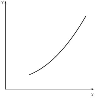
\[ P \equiv \frac{\partial Y}{\partial X} \]
is the slope of this curve. Now, if we desire to consider \(P\) as an independent variable in place of \(X\), our first impulse might be simply to eliminate \(X\) between equations 5.15 and 5.16, thereby obtaining \(Y\) as a function of \(P\)
\[ Y=Y(P) \]
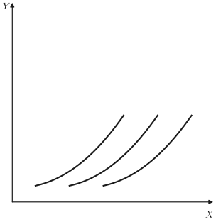
A moment’s reflection indicates, however, that we would sacrifice some of the mathematical content of the given fundamental relation (5.15) for, from the geometrical point of view, it is clear that knowledge of \(Y\) as a function of the slope \(d Y / d X\) would not permit us to reconstruct the curve \(Y=Y(X)\). In fact, each of the displaced curves shown in Fig. 5.4 corresponds equally well to the relation \(Y=Y(P)\). From the analytical point of view the relation \(Y=Y(P)\) is a first-order differential equation, and its integration gives \(Y=Y(X)\) only to within an undetermined integration constant. Therefore we see that acceptance of \(Y=Y(P)\) as a basic equation in place of \(Y=Y(X)\) would involve the sacrifice of some information originally contained in the fundamental relation. Despite the
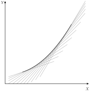
The practicable solution to the problem is supplied by the duality between conventional point geometry and the Pluecker line geometry. The essential concept in line geometry is that a given curve can be represented equally well either \((a)\) as the envelope of a family of tangent lines (Fig. 5.5), or ( \(b\) ) as the locus of points satisfying the relation \(Y=Y(X)\). Any equation that enables us to construct the family of tangent lines therefore determines the curve equally as well as the relation \(Y=Y(X)\).
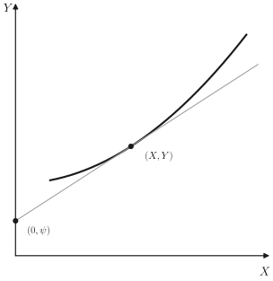
Just as every point in the plane is described by the two numbers \(X\) and \(Y\), so every straight line in the plane can be described by the two numbers \(P\) and \(\psi\), where \(P\) is the slope of the line and \(\psi\) is its intercept along the \(Y\)-axis. Then just as a relation \(Y=Y(X)\) selects a subset of all possible points ( \(X, Y\) ), a relation \(\psi=\psi(P)\) selects a subset of all possible lines \((P, \psi)\). A knowledge of the intercepts \(\psi\) of the tangent lines as a function of the slopes \(P\) enables us to construct the family of tangent lines and thence the curve of which they are the envelope. Thus the relation
\[ \psi=\psi(P) \]
is completely equivalent to the fundamental relation \(Y=Y(X)\). In this relation the independent variable is \(P\), so that equation 5.18 provides a complete and satisfactory solution to the problem. As the relation \(\psi=\) \(\psi(P)\) is mathematically equivalent to the relation \(Y=Y(X)\), it can also be considered a fundamental relation; \(Y=Y(X)\) is a fundamental relation in the ” \(Y\)-representation”; whereas \(\psi=\psi(P)\) is a fundamental relation in the ” \(\psi\)-representation.”
The reader is urged at this point actually to draw a reasonable number of straight lines, of various slopes \(P\) and of various \(Y\)-intercepts \(\psi=-P^{2}\). The relation \(\psi=-P^{2}\) thereby will be seen to characterize a parabola (which is more conventionally described as \(Y=\frac{1}{4} X^{2}\) ). In \(\psi\)-representation the fundamental equation of the parabola is \(\psi=-P^{2}\), whereas in \(Y\)-representation the fundamental equation of this same parabola is \(Y=\frac{1}{4} X^{2}\).
The question now arises as to how we can compute the relation \(\psi=\psi(P)\) if we are given the relation \(Y=Y(X)\). The appropriate mathematical operation is known as a Legendre transformation. We consider a tangent line that goes through the point \((X, Y)\) and has a slope \(P\). If the intercept is \(\psi\), we have (see Fig. 5.6)
\[ P=\frac{Y-\psi}{X-0} \]
or
\[ \psi=Y-P X \]
Let us now suppose that we are given the equation
\[ Y=Y(X) \]
\[ P=P(X) \]
Then by elimination \({ }^{1}\) of \(X\) and \(Y\) among equations 5.20, 5.21, and 5.22 we obtain the desired relation between \(\psi\) and \(P\). The basic identity of the Legendre transformation is equation 5.20, and this equation can be taken as the analytic definition of the function \(\psi\). The function \(\psi\) is referred to as a Legendre transform of \(Y\).
The inverse problem is that of recovering the relation \(Y=Y(X)\) if the relation \(\psi=\psi(P)\) is given. We shall see here that the relationship between \((X, Y)\) and \((P, \psi)\) is symmetrical with its inverse, except for a sign in the equation of the Legendre transformation. Taking the differential of equation 5.20 and recalling that \(d Y=P d X\), we find
\[ \begin{aligned} d \psi & =d Y-P d X-X d P \\ & =-X d P \end{aligned} \]
or
\[ -X=\frac{d \psi}{d P} \]
If the two variables \(\psi\) and \(P\) are eliminated \({ }^{2}\) from the given equation \(\psi=\psi(P)\) and from equations 5.24 and 5.20, we recover the relation \(Y=Y(X)\). The symmetry between the Legendre transformation and its inverse is indicated by the following schematic comparison:
| \(Y=Y(X)\) | \(\psi=\psi(P)\) |
|---|---|
| \(P=\frac{d Y}{d X}\) | \(-X=\frac{d \psi}{d P}\) |
| \(\psi=-P X+Y\) | \(Y=X P+\psi\) |
| Elimination of \(X\) and \(Y\) yields \(\psi=\psi(P)\) | Elimination of \(P\) and \(\psi\) yields \(Y=Y(X)\) |
[^13]satisfying the fundamental equation \(Y=Y\left(X_{0}, X_{1}\right)\), or it can be considered as the envelope of tangent planes. A plane can be characterized by its intercept \(\psi\) on the \(Y\)-axis and by the slopes \(P_{0}\) and \(P_{1}\) of its traces on the \(Y-X_{0}\) and \(Y-X_{1}\) planes. The fundamental equation then selects from all possible planes a subset described by \(\psi=\psi\left(P_{0}, P_{1}\right)\).
In general the given fundamental relation
\[ Y=Y\left(X_{0}, X_{1}, \ldots, X_{t}\right) \]
represents a hypersurface in a \((t+2)\)-dimensional space with cartesian coordinates \(Y, X_{0}, X_{1}, \ldots, X_{t}\). The derivative
\[ P_{k}=\frac{\partial Y}{\partial X_{k}} \]
is the partial slope of this hypersurface. The hypersurface may be equally well represented as the locus of points satisfying equation 5.25 or as the envelope of the tangent hyperplanes. The family of tangent hyperplanes can be characterized by giving the intercept of a hyperplane, \(\psi\), as a function of the slopes \(P_{0}, P_{1}, \ldots, P_{t}\). Then
\[ \psi=Y-\sum_{k} P_{k} X_{k} \]
Taking the differential of this equation, we find
\[ d \psi=-\sum_{k} X_{k} d P_{k} \]
whence
\[ -X_{k}=\frac{\partial \psi}{\partial P_{k}} \]
A Legendre transformation is effected by eliminating \(Y\) and the \(X_{k}\) from \(Y=Y\left(X_{0}, X_{1}, \ldots, X_{t}\right)\), the set of equations 5.26, and equation 5.27. The inverse transformation is effected by eliminating \(\psi\) and the \(P_{k}\) from \(\psi=\psi\left(P_{1}, P_{2}, \ldots, P_{r}\right)\), the set of equations 5.29, and equation 5.27.
Finally, a Legendre transformation may be made only in some \((n+2)\) dimensional subspace of the full \((t+2)\)-dimensional space of the relation \(Y=Y\left(X_{0}, X_{1}, \ldots, X_{t}\right)\). Of course the subspace must contain the \(Y\)-coordinate but may involve any choice of \(n+1\) coordinates from the set \(X_{0}, X_{1}, \ldots, X_{t}\). For convenience of notation, we order the coordinates so that the Legendre transformation is made in the subspace of the first \(n+1\) coordinates (and of \(Y\) ); the coordinates \(X_{n+1}, X_{n+1}, \ldots . X\) are left untransformed. Such a partial Legendre transformation is effected merely by considering the variables \(X_{n+1}, X_{n+2}, \ldots, X_{t}\) as constants in the transformation. The resulting Legendre transform must be denoted by some explicit notation that indicates which of the independent variables have participated in the transformation. We employ the notation \(Y\left[P_{0}, P_{1}, \ldots, P_{n}\right]\) to denote the function obtained by making a Legendre transformation with respect to \(X_{0}, X_{1}, \ldots, X_{n}\) on the function \(Y\left(X_{0}, X_{1}, \ldots, X_{t}\right)\). Thus \(Y\left[P_{0}, P_{1}, \ldots, P_{n}\right]\) is a function of the independent variables \(P_{0}, P_{1}, \ldots, P_{n}, X_{n+1}, \ldots, X_{r}\). The various relations involved in a partial Legendre transformation and its inverse are indicated in the following table.
\[ \begin{aligned} Y & =Y\left(X_{0}, X_{1}, \ldots, X_{t}\right) \\ P_{k} & =\frac{\partial Y}{\partial X_{k}} \end{aligned} \]
The partial differentiation denotes constancy of all the natural variables of \(Y\) other than \(X_{k}\) (i.e., of all \(X_{j}\) with \(j \neq k\) )
\[ d Y=\sum_{0}^{t} P_{k} d X_{k} \]
\[ Y\left[P_{0}, \ldots, P_{n}\right]=Y-\sum_{0}^{n} P_{k} X_{k} \]
Elimination of \(Y\) and \(X_{0}\), \(X_{1}, \ldots, X_{n}\) from equations 5.30, 5.33, and the first \(n+1\) equations of 5.31 yields the transformed fundamental relation. \(Y\left[P_{0}, P_{1}, \ldots, P_{n}\right]=\) function of \(P_{0}, P_{1}, \ldots, P_{n}, X_{n+1}, \ldots, X_{t}\)
\[ -X_{k}=\frac{\partial Y\left[P_{0}, \ldots, P_{n}\right]}{\partial P_{k}} \quad k \leq n \]
\[ P_{k}=\frac{\partial Y\left[P_{0}, \ldots, P_{n}\right]}{\partial X_{k}} \quad k>n \]
The partial differentiation denotes constancy of all the natural variables of \(Y\left(P_{0}, \ldots, P_{n}\right)\) other than that with respect to which the differentiation is being carried out.
\[ \begin{aligned} & d Y\left[P_{0}, \ldots, P_{n}\right] \\ & \quad=-\sum_{0}^{n} X_{k} d P_{k}+\sum_{n+1}^{t} P_{k} d X_{k} \end{aligned} \]
\[ Y=Y\left[P_{0}, \ldots, P_{n}\right]+\sum_{0}^{n} X_{k} P_{k} \]
Elimination of \(Y\left[P_{0}, \ldots, P_{n}\right]\) and \(P_{0}, P_{1}, \ldots, P_{n}\) from equations 5.30, 5.33, and the first \(n+1\) equations of 5.31 yields the original fundamental relation.
In this section we have divorced the mathematical aspects of Legendre transformations from the physical applications. Before proceeding to the thermodynamic applications in the succeeding sections of this chapter, it may be of interest to indicate very briefly the application of the formalism to Lagrangian and Hamiltonian mechanics, which perhaps may be a more familiar field of physics than thermodynamics. The Lagrangian principle guarantees that a particular function, the Lagrangian, completely characterizes the dynamics of a mechanical system. The Lagrangian is a function of \(2 r\) variables, \(r\) of which are generalized coordinates and \(r\) of which are generalized velocities. Thus the equation
\[ L=L\left(v_{1}, v_{2}, \ldots, v_{r}, q_{1}, q_{2}, \ldots, q_{r}\right) \]
plays the role of a fundamental relation. The generalized momenta are defined as derivatives of the Lagrangian function
\[ P_{k} \equiv \frac{\partial L}{\partial v_{k}} \]
If it is desired to replace the velocities by the momenta as independent variables, we must make a partial Legendre transformation with respect to the velocities. We thereby introduce a new function, called the Hamiltonian, defined by \({ }^{3}\)
\[ (-H)=L-\sum_{1}^{r} P_{k} v_{k} \]
A complete dynamical formalism can then be based on the new fundamental relation
\[ H=H\left(P_{1}, P_{2}, \ldots, P_{r}, q_{1}, q_{2}, \ldots, q_{r}\right) \]
Furthermore, by equation 5.31 the derivative of \(H\) with respect to \(P_{k}\) is the velocity \(v_{k}\), which is one of the Hamiltonian dynamical equations. Thus, if an equation of the form 5.34 is considered as a dynamical fundamental equation in the Lagrangian representation, the Hamiltonian equation (5.37) is the equivalent fundamental equation expressed in the Hamiltonian representation.
PROBLEMS
Problem 5.2-1
The equation \(y=x^{2} / 10\) describes a parabola.
Find the equation of this parabola in the “line geometry representation” \(\psi=\psi(P)\).
On a sheet of graph paper (covering the range roughly from \(x \simeq-15\) to \(x \simeq+15\) and from \(y \simeq-25\) to \(y \simeq+25\) ) draw straight lines with slopes \(P=0\),
[^14]\(\pm 0.5, \pm 1, \pm 2, \pm 3\) and with intercepts \(\psi\) satisfying the relationship \(\psi=\psi(P)\) as found in part (a). (Drawing each straight line is facilitated by calculating its intercepts on the \(x\)-axis and on the \(y\)-axis.)
Problem 5.2-2
Let \(y=A e^{B x}\).
a)Find \(\psi(P)\). b)Calculate the inverse Legendre transform of \(\psi(P)\) and corroborate that this result is \(y(x)\). c)Taking \(A=2\) and \(B=0.5\), draw a family of tangent lines in accordance with the result found in \((a)\), and check that the tangent curve goes through the expected points at \(x=0,1\), and 2 .
5-3 THERMODYNAMIC POTENTIALS
The application of the preceding formalism to thermodynamics is self-evident. The fundamental relation \(Y=Y\left(X_{0}, X_{1}, \ldots\right)\) can be interpreted as the energy-language fundamental relation \(U=U(S\), \(\left.X_{1}, X_{2}, \ldots, X_{t}\right)\) or \(U=U\left(S, V, N_{1}, N_{2}, \ldots\right)\). The derivatives \(P_{0}, P_{1}, \ldots\) correspond to the intensive parameters \(T,-P, \mu_{1}, \mu_{2}, \ldots\). The Legendre transformed functions are called thermodynamic potentials, and we now specifically define several of the most common of them. In Chapter 6 we continue the discussion of these functions by deriving extremum principles for each potential, indicating the intuitive significance of each, and discussing its particular role in thermodynamic theory. But for the moment we concern ourselves merely with the formal aspects of the definitions of the several particular functions.
The Helmholtz potential or the Helmholtz free energy, is the partial Legendre transform of \(U\) that replaces the entropy by the temperature as the independent variable. The internationally adopted symbol for the Helmholtz potential is \(F\). The natural variables of the Helmholtz potential are \(T, V, N_{1}, N_{2}, \ldots\). That is, the functional relation \(F=\) \(F\left(T, V, N_{1}, N_{2}, \ldots\right)\) constitutes a fundamental relation. In the systematic notation introduced in Section 5.2
\[ F \equiv U[T] \]
The full relationship between the energy representation and the Helmholtz representation, is summarized in the following schematic comparison:
| \(U=U\left(S, V, N_{1}, N_{2}, \ldots\right)\) | \(F=F\left(T, V, N_{1}, N_{2}, \ldots\right)\) | (5.39) |
|---|---|---|
| \(T=\partial U / \partial S\) | \(-S=\partial F / \partial T\) | (5.40) |
| \(F=U-T S\) | \(U=F+T S\) | (5.41) |
| Elimination of \(U\) and \(S\) yields \(F=F\left(T, V, N_{1}, N_{2}, \ldots\right)\) | Elimination of \(F\) and \(T\) yields \(U=U\left(S, V, N_{1}, N_{2}, \ldots\right)\) |
The complete differential \(d F\) is
\[ d \boldsymbol{F}=-\boldsymbol{S} d \boldsymbol{T}-\boldsymbol{P} d \boldsymbol{V}+\mu_{1} d N_{1}+\mu_{2} d N_{2}+\cdots \]
The enthalpy is that partial Legendre transform of \(U\) that replaces the volume by the pressure as an independent variable. Following the recommendations of the International Unions of Physics and of Chemistry, and in agreement with almost universal usage, we adopt the symbol \(H\) for the enthalpy. The natural variables of this potential are \(S, P, N_{1}, N_{2}, \ldots\) and
\[ H \equiv U[P] \]
The schematic representation of the relationship of the energy and enthalpy representations is as follows:
| \(U=U\left(S, V, N_{1}, N_{2}, \ldots\right)\) | \(H=H\left(S, P, N_{1}, N_{2}, \ldots\right)\) | (5.44) |
|---|---|---|
| \(-P=\partial U / \partial V\) | \(V=\partial H / \partial P\) | (5.45) |
| \(H=U+P V\) | \(U=H-P V\) | (5.46) |
| Elimination of \(U\) and \(V\) yields \(H=H\left(S, P, N_{1}, N_{2}, \ldots\right)\) | Elimination of \(H\) and \(P\) yields \(U=U\left(S, V, N_{1}, N_{2}, \ldots\right)\) |
Particular attention is called to the inversion of the signs in equations 5.45 and 5.46 , resulting from the fact that \(-P\) is the intensive parameter associated with \(V\). The complete differential \(d H\) is
\[ d H=T d S+V d P+\mu_{1} d N_{1}+\mu_{2} d N_{2}+\cdots \]
The third of the common Legendre transforms of the energy is the Gibbs potential, or Gibbs free energy. This potential is the Legendre transform that simultaneously replaces the entropy by the temperature and the volume by the pressure as independent variables. The standard notation is \(G\), and the natural variables are \(T, P, N_{1}, N_{2}, \ldots\). We thus have
\[ G \equiv U[T, P] \]
and
| \(U=U\left(S, V, N_{1}, N_{2}, \ldots\right)\) | \(G=G\left(T, P, N_{1}, N_{2}, \ldots\right)\) |
|---|---|
| \(T=\partial U / \partial S\) | \(-S=\partial G / \partial T\) |
| \(-P=\partial U / \partial V\) | \(V=\partial G / \partial P\) |
| \(G=U-T S+P V\) | \(U=G+T S-P V\) |
| Elimination of \(U, S\), and \(V\) yields \(G=G\left(T, P, N_{1}, N_{2}, \ldots\right)\) | Elimination of \(G, T\), and \(P\) yields \(U=U\left(S, V, N_{1}, N_{2}, \ldots\right)\) |
The complete differential \(d G\) is
\[ d G=-S d T+V d P+\mu_{1} d N_{1}+\mu_{2} d N_{2}+\cdots \]
A thermodynamic potential which arises naturally in statistical mechanics is the grand canonical potential, \(U[T, \mu]\). For this potential we have
| \(U=U(S, V, N)\) | \(U[T, \mu]=\) function of \(T, V\), and \(\mu\) (5.54) |
|---|---|
| \(T=\partial U / \partial S\) | \(-S=\partial U[T, \mu] / \partial T\) |
| \(\mu=\partial U / \partial N\) | \(-N=\partial U[T, \mu] / \partial \mu\) |
| \(U[T, \mu]=U-T S-\mu N\) | \(U=U[T, \mu]+T S+\mu N\) |
| Elimination of | Elimination of |
| \(U, S\), and \(N\) yields | \(U[T, \mu], T\), and \(\mu\) yields |
| \(U[T, \mu]\) as a function of \(T, V, \mu\) | \(U=U(S, V, N)\) |
and
\[ d U[T, \mu]=-S d T-P d V-N d \mu \]
Other possible transforms of the energy for a simple system, which are used only infrequently and which consequently are unnamed, are \(U\left[\mu_{1}\right]\), \(U\left[P, \mu_{1}\right], U\left[T, \mu_{1}, \mu_{2}\right]\), and so forth. The complete Legendre transform is \(U\left[T, P, \mu_{1}, \mu_{2}, \ldots, \mu_{r}\right]\). The fact that \(U\left(S, V, N_{1}, N_{2}, \ldots, N_{i}\right)\) is a homogeneous first-order function of its arguments causes this latter function to vanish identically. For
\[ U\left[T, P, \mu_{1}, \ldots, \mu_{r}\right]=U-T S+P V-\mu_{1} N_{1}-\mu_{2} N_{2}-\cdots-\mu_{r} N_{r} \]
which, by the Euler relation (3.6), is identically zero
\[ U\left[T, P, \mu_{1}, \ldots, \mu_{r}\right] \equiv 0 \]
PROBLEMS
Problem 5.3-1
Find the fundamental equation of a monatomic ideal gas in the Helmholtz representation, in the enthalpy representation, and in the Gibbs representation. Assume the fundamental equation computed in Section 3.4. In each case find the equations of state by differentiation of the fundamental equation.
Problem 5.3-2
Find the fundamental equation of the ideal van der Waals fluid (Section \(3.5)\) in the Helmholtz representation.
Perform an inverse Legendre transform on the Helmholtz potential and show that the fundamental equation in the energy representation is recovered.
Problem 5.3-3
Find the fundamental equation of electromagnetic radiation in the Helmholtz representation. Calculate the “thermal” and “mechanical” equations of state and corroborate that they agree with those given in Section 3.6.
5.3-4 \({ }^{4}\). Justify the following recipe for obtaining a plot of \(F(V)\) from a plot of \(G(P)\) (the common dependent variables \(T\) and \(N\) being notationally suppressed for convenience). 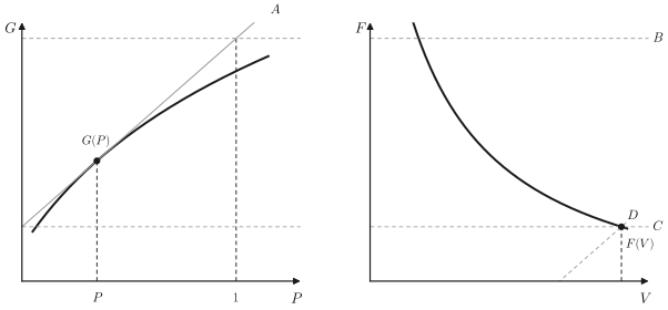 (1) At a chosen value of \(P\) draw the tangent line \(A\). (2) Draw horizontal lines \(\boldsymbol{B}\) and \(\boldsymbol{C}\) through the intersections of \(A\) with \(P=1\) and \(P=0\). (3) Draw the 45° line \(D\) as shown and project the intersection of \(B\) and \(D\) onto the line \(C\) to obtain the point \(F(V)\). Hint: Identify the magnitude of the two vertical distances indicated in the \(G\) versus \(P\) diagram, and also the vertical separation of lines \(B\) and \(C\).
Note that the units of \(F\) and \(V\) are determined by the chosen units of \(G\) and \(P\). Explain.
Give the analogous construction for at least one other pair of potentials. Note that \(G(P)\) is drawn as a concave function (i.e., negative curvature) and show that this is equivalent to the statement that \(\kappa_{T}>0\).
Problem 5.3-5
From the first acceptable fundamental equation in Problem 1.10-1 calculate the fundamental equation in Gibbs representation. Calculate \(\alpha(T, P)\), \(\kappa_{T}(T, P)\), and \(c_{p}(T, P)\) by differentiation of \(G\).
Problem 5.3-6
From the second acceptable fundamental equation in Problem 1.10-1 calculate the fundamental equation in enthalpy representation. Calculate \(V(S, P, N)\) by differentiation.
Problem 5.3-7
The enthalpy of a particular system is
\[ H=A S^{2} N^{-1} \ln \left(\frac{P}{P_{0}}\right) \]
[^15]where \(A\) is a positive constant. Calculate the molar heat capacity at constant volume \(c_{v}\) as a function of \(T\) and \(P\).
Problem 5.3-8
In Chapter 15 it is shown by a statistical mechanical calculation that the fundamental equation of a system of \(\tilde{N}\) “atoms” each of which can exist in an atomic state with energy \(\varepsilon_{u}\) or in an atomic state with energy \(\varepsilon_{d}\) (and in no other state) is
\[ F=-\bar{N} k_{B} T^{\ln }\left(e^{-\beta \varepsilon_{u}}+e^{-\beta \varepsilon_{d}}\right) \] Here \(k_{B}\) is Boltzmann’s constant and \(\beta=1 / k_{B} T\). Show that the fundamental equation of this system, in entropy representation, is \[ S=N R \ln \left(\frac{1+Y^{\varepsilon_{d} / \varepsilon_{u}}}{Y^{Y}}\right) \] where \[ Y \equiv \frac{U-\tilde{N} \varepsilon_{u}}{\bar{N} \varepsilon_{d}-U} \]
Hint: Introduce \(\beta=\left(k_{B} T\right)^{-1}\), and show first that \(U=F+\beta \partial F / \partial \beta=\) \(\partial(\beta F) / \partial \beta\). Also, for definiteness, assume \(\varepsilon_{u}<\varepsilon_{d}\), and note that \(\bar{N} k_{B}=N R\) where \(\bar{N}\) is the number of atoms and \(N\) is the number of moles.
Problem 5.3-9
Show, for the two-level system of Problem 5.3-8, that as the temperature increases from zero to infinity the energy increases from \(\tilde{N} \varepsilon_{u}\) to \(\tilde{N}\left(\varepsilon_{u}+\varepsilon_{d}\right) / 2\). Thus, at zero temperature all atoms are in their “ground state” (with energy \(\varepsilon_{u}\) ), and at infinite temperature the atoms are equally likely to be in either state. Energies higher than \(N\left(\varepsilon_{u}+\varepsilon_{d}\right) / 2\) are inaccessible in thermal equilibrium! (This upper bound on the energy is a consequence of the unphysical oversimplification of the model; it will be discussed again in Section 15.3.)
Show that the Helmholtz potential of a mixture of simple ideal gases is the sum of the Helmholtz potentials of each individual gas: 5.3-10.
- Show that the Helmholtz potential of a mixture of simple ideal gases is the sum of the Helmholtz potentials of each individual gas:
\[ F\left(T, V, N_{1}, \ldots, N_{r}\right)=F\left(T, V, N_{1}\right)+\cdots+F\left(T, V, N_{r}\right) \]
Recall the fundamental equation of the mixture, as given in equation 3.40. An analogous additivity does not hold for any other potential expressed in terms of its natural variables.
Problem 5.3-11
A mixture of two monatomic ideal gases is contained in a volume \(V\) at temperature \(T\). The mole numbers are \(N_{1}\) and \(N_{2}\). Calculate the chemical potentials \(\mu_{1}\) and \(\mu_{2}\). Recall Problems 5.3-1 and 5.3-10.
Assuming the system to be in contact with a reservoir of given \(T\) and \(\mu_{1}\), through a diathermal wall permeable to the first component but not to the second, calculate the pressure in the system.
Problem 5.3-12
A system obeys the fundamental relation
\[ \left(s-s_{0}\right)^{4}=A v u^{2} \]
Calculate the Gibbs potential \(G(T, P, N)\).
Problem 5.3-13
For a particular system it is found that
\[ u=\left(\frac{3}{2}\right) P v \]
and
\[ P=A v T^{4} \]
Find a fundamental equation, the molar Gibbs potential, and the Helmholtz potential for this system.
Problem 5.3-14
For a particular system (of 1 mole) the quantity \((v+a) f\) is known to be a function of the temperature only \((=\boldsymbol{Y}(\boldsymbol{T}))\). Here \(\boldsymbol{v}\) is the molar volume, \(f\) is the molar Helmholtz potential, \(a\) is a constant, and \(Y(T)\) denotes an unspecified function of temperature. It is also known that the molar heat capacity \(c_{v}\) is
\[ c_{v}=b(v) T^{\frac{1}{2}} \]
where \(b(v)\) is an unspecified function of \(v\).
Evaluate \(Y(T)\) and \(b(v)\).
The system is to be taken from an initial state ( \(T_{0}, v_{0}\) ) to a final state ( \(T_{f}, v_{f}\) ). A thermal reservoir of temperature \(T_{r}\) is available, as is a reversible work source. What is the maximum work that can be delivered to the reversible work source? (Note that the answer may involve constants unevaluated by the stated conditions, but that the answer should be fully explicit otherwise.)
5-4 GENERALIZED MASSIEU FUNCTIONS
Whereas the most common functions definable in terms of Legendre transformations are those mentioned in Section 5.3, another set can be defined by performing the Legendre transformation on the entropy rather than on the energy. That is, the fundamental relation in the form \(S=\) \(S\left(U, V, N_{1}, N_{2}, \ldots\right)\) can be taken as the relation on which the transformation is performed. Such Legendre transforms of the entropy were invented by Massieu in 1869 and actually predated the transforms of the energy introduced by Gibbs in 1875. We refer to the transforms of the entropy as Massieu functions, as distinguished from the thermodynamic potentials transformed from the energy. The Massieu functions will turn out to be particularly useful in the theory of irreversible thermodynamics, and they also arise naturally in statistical mechanics and in the theory of thermal fluctuations. Three representative Massieu functions are \(S[1 / T]\), in which the internal energy is replaced by the reciprocal temperature as independent variable; \(S[P / T]\), in which the volume is replaced by \(P / T\) as independent variable; and \(S[1 / T, P / T]\), in which both replacements are made simultaneously. Clearly
\[ \begin{aligned} & S\left[\frac{1}{T}\right] \equiv S-\frac{1}{T} U=-\frac{F}{T} \\ & S\left[\frac{P}{T}\right] \equiv S-\frac{P}{T} \cdot V \end{aligned} \]
and
\[ S\left[\frac{1}{T}, \frac{P}{T}\right]=S-\frac{1}{T} U-\frac{P}{T} \cdot V=-\frac{G}{T} \]
Thus, of the three, only \(S[P / T]\) is not trivially related to one of the previously introduced thermodynamic potentials. For this function
| \(S=S\left(U, V, N_{1}, N_{2}, \ldots\right)\) | \(S[P / T]=\) function of \(U, P / T, N_{1}, N_{2}, \ldots, \text { (5.64) }\) |
|---|---|
| \(P / T=\partial S / \partial V\) \(S[P / T]=S-(P / T) V\) | \(-V=\partial S[P / T] / \partial(P / T)\) (5.65) \(S=S[P / T]+(P / T) V(5.66)\) |
| Elimination of | Elimination of |
| \(S\) and \(V\) yields \(S[P / T]\) as a function of \(U, P / T, N_{1}, N_{2}, \ldots\) | \(S[P / T]\) and \(P / T\) yields \(S=S\left(U, V, N_{1}, N_{2}, \ldots\right)\) |
and
\[ d S[P / T]=(1 / T) d U-V d(P / T)-\left(\mu_{1} / T\right) d N_{1}-\frac{\mu_{2}}{T} d N_{2} \ldots \]
Other Massieu functions may be invented and analyzed by the reader as a particular need for them arises.
PROBLEMS
Problem 5.4-1
Find the fundamental equation of a monatomic ideal gas in the representation
\[ S\left[\frac{P}{T}, \frac{\mu}{T}\right] \]
Find the equations of state by differentiation of this fundamental equation.
Problem 5.4-2
Find the fundamental equation of electromagnetic radiation (Section 3.6)
in the representation \(S[1 / T]\)
in the representation \(S[P / T]\)
Problem 5.4-3
Find the fundamental equation of the ideal van der Waals fluid in the representation \(S[1 / T]\). Show that \(S[1 / T]\) is equal to \(-F / T\) (recall that \(F\) was computed in Problem 5.3-2).