THE EXTREMUM PRINCIPLE IN THE LEGENDRE TRANSFORMED REPRESENTATIONS
6-1 THE MINIMUM PRINCIPLES FOR THE POTENTIALS
We have seen that the Legendre transformation permits expression of the fundamental equation in terms of a set of independent variables chosen to be particularly convenient for a given problem. Clearly, however, the advantage of being able to write the fundamental equation in various representations would be lost if the extremum principle were not itself expressible in those representations. We are concerned, therefore, with the reformulation of the basic extremum principle in forms appropriate to the Legendre transformed representations.
For definiteness consider a composite system in contact with a thermal reservoir. Suppose further that some internal constraint has been removed. We seek the mathematical condition that will permit us to predict the equilibrium state. For this purpose we first review the solution of the problem by the energy minimum principle.
In the equilibrium state the total energy of the composite system-plusreservoir is minimum:
\[ d\left(U+U^{r}\right)=0 \]
and
\[ d^{2}\left(U+U^{r}\right)=d^{2} U>0 \]
subject to the isentropic condition
\[ d\left(S+S^{r}\right)=0 \]
The quantity \(d^{2} U^{r}\) has been put equal to zero in equation 6.2 because \(d^{2} U^{r}\) is a sum of products of the form
\[ \frac{\partial^{2} U^{r}}{\partial X_{j}^{r} \partial X_{k}^{r}} d X_{j}^{r} d X_{k}^{r} \]
which vanish for a reservoir (the coefficient varying as the reciprocal of the mole number of the reservoir).
The other closure conditions depend upon the particular form of the internal constraints in the composite system. If the internal wall is movable and impermeable, we have
\[ d N_{j}^{(1)}=d N_{,}^{(2)}=d\left(V^{(1)}+V^{(2)}\right)=0 \quad(\text { for all } j) \]
whereas, if the internal wall is rigid and permeable to the \(k\) th component, we have
\[ d\left(N_{k}^{(1)}+N_{k}^{(2)}\right)=d N_{j}^{(1)}=d N_{j}^{(2)}=d V^{(1)}=d V^{(2)}=0 \quad(j \neq k) \]
These equations suffice to determine the equilibrium state. The differential \(d U\) in equation 6.1 involves the terms \(T^{(1)} d S^{(1)}+\) \(T^{(2)} d S^{(2)}\), which arise from heat flux among the subsystems and the reservoir, and terms such as \(-P^{(1)} d V^{(1)}-P^{(2)} d V^{(2)}\) and \(\mu_{k}^{(1)} d N_{k}^{(1)}+\) \(\mu_{k}^{(2)} d N_{k}^{(2)}\), which arise from processes within the composite system. The terms \(T^{(1)} d S^{(1)}+T^{(2)} d S^{(2)}\) combine with the term \(d U^{r}=T^{r} d S^{r}\) in equation 6.1 to yield
\[ \begin{aligned} T^{(1)} d S^{(1)}+T^{(2)} d S^{(2)}+T^{r} d S^{r} & =T^{(1)} d S^{(1)}+T^{(2)} d S^{(2)}-T^{r} d\left(S^{(1)}+S^{(2)}\right) \\ & =0 \end{aligned} \]
whence
\[ T^{(1)}=T^{(2)}=T^{r} \]
Thus one evident aspect of the final equilibrium state is the fact that the reservoir maintains a constancy of temperature throughout the system. The remaining conditions of equilibrium naturally depend upon the specific form of the internal constraints in the composite system.
To this point we have merely reviewed the application of the energy minimum principle to the composite system (the subsystem plus the reservoir). We are finally ready to recast equations 6.1 and 6.2 into the language of another representation. We rewrite equation 6.1
\[ d\left(U+U^{r}\right)=d U+T^{r} d S^{r}=0 \]
or, by equation 6.3
\[ d U-T^{r} d S=0 \]
or, further, since \(T^{r}\) is a constant
\[ d\left(U-T^{r} S\right)=0 \]
Similarly, since \(T^{r}\) is a constant and \(S\) is an independent variable, equation 6.2 implies \({ }^{1}\)
\[ d^{2} U=d^{2}\left(U-T^{r} S\right)>0 \]
Thus the quantity ( \(U-T^{r} S\) ) is minimum in the equilibrium state. Now the quantity \(U-T^{r} S\) is suggestive by its form of the Helmholtz potential \(U-T S\). We are therefore led to examine further the extremum properties of the quantity ( \(U-T^{r} S\) ) and to ask how these may be related to the extremum properties of the Helmholtz potential. We have seen that an evident feature of the equilibrium is that the temperature of the composite system (i.e., of each of its subsystems) is equal to \(T^{r}\). If we accept that part of the solution, we can immediately restrict our search for the equilibrium state among the manifold of states for which \(T=T^{r}\). But over this manifold of states \(U-T S\) is identical to \(U-T^{r} S\). Then we can write equation 6.10 as
\[ d F=d(U-T S)=0 \]
subject to the auxiliary condition that
\[ T=T^{r} \]
That is, the equilibrium state minimizes the Helmholtz potential, not absolutely, but over the manifold of states for which \(T=T^{r}\). We thus arrive at the equilibrium condition in the Helmholtz potential representation. Helmholtz Potential Minimum Principle. The equilibrium value of any unconstrained internal parameter in a system in diathermal contact with a heat reservoir minimizes the Helmholtz potential over the manifold of states for which \(T=T^{r}\).
[^16]The intuitive significance of this principle is clearly evident in equations 6.8 through 6.10 . The energy of the system plus the reservoir is, of course, minimum. But the statement that the Helmholtz potential of the system alone is minimum is just another way of saying this, for \(d F=d(U-T S)\), and the term \(d(-T S)\) actually represents the change in energy of the reservoir (since \(T=T^{r}\) and \(-d S=d S^{r}\) ). It is now a simple matter to extend the foregoing considerations to the other common representations.
Consider a composite system in which all subsystems are in contact with a common pressure reservoir through walls nonrestrictive with respect to volume. We further assume that some internal constraint within the composite system has been removed. The first condition of equilibrium can be written
\[ d\left(U+U^{r}\right)=d U-P^{r} d V^{r}=d U+P^{r} d V=0 \]
or
\[ d\left(U+P^{r} V\right)=0 \]
Accepting the evident condition that \(P=P^{r}\), we can write
\[ d H=d(U+P V)=0 \]
subject to the auxiliary restriction
\[ P=P^{r} \]
Furthermore, since \(P^{r}\) is a constant and \(V\) is an independent variable
\[ d^{2} H=d^{2}\left(U+P^{r} V\right)=d^{2} U>0 \]
so that the extremum is a minimum. Enthalpy Minimum Principle. The equilibrium value of any unconstrained internal parameter in a system in contact with a pressure reservoir minimizes the enthalpy over the manifold of states of constant pressure (equal to that of the pressure reservoir).
Finally, consider a system in simultaneous contact with a thermal and a pressure reservoir. Again
\[ d\left(U+U^{r}\right)=d U-T^{r} d S+P^{r} d V=0 \]
Accepting the evident conditions that \(T=T^{r}\) and \(P=P^{r}\), we can write
\[ d G=d(U-T S+P V)=0 \]
subject to the auxiliary restrictions
\[ T=T^{r} \quad P=P^{r} \]
Again
\[ d^{2} G=d^{2}\left(U-T^{r} S+P^{r} V\right)=d^{2} U>0 \]
We thus obtain the equilibrium condition in the Gibbs representation. Gibbs Potential Minimum Principle. The equilibrium value of any unconstrained internal parameter in a system in contact with a thermal and a pressure reservoir minimizes the Gibbs potential at constant temperature and pressure (equal to those of the respective reservoirs).
If the system is characterized by other extensive parameters in addition to the volume and the mole numbers the analysis is identical in form and the general result is now clear:
The General Minimum Principle for Legendre Transforms of the Energy. The equilibrium value of any unconstrained internal parameter in a system in contact with a set of reservoirs (with intensive parameters \(P_{1}^{r}, P_{2}^{r}, \ldots\) ) minimizes the thermodynamic potential \(U\left[P_{1}, P_{2}, \ldots\right]\) at constant \(P_{1}, P_{2}, \ldots\) (equal to \(P_{1}^{r}, P_{2}^{r}, \ldots\) ).
6-2 THE HELMHOLTZ POTENTIAL
For a composite system in thermal contact with a thermal reservoir the equilibrium state minimizes the Helmholtz potential over the manifold of states of constant temperature (equal to that of the reservoir). In practice many processes are carried out in rigid vessels with diathermal walls, so that the ambient atmosphere acts as a thermal reservoir; for these the Helmholtz potential representation is admirably suited.
The Helmholtz potential is a natural function of the variables \(T, V, N_{1}, N_{2}, \ldots\). The condition that \(T\) is constant reduces the number of variables in the problem, and \(F\) effectively becomes a function only of the variables \(V\) and \(N_{1}, N_{2}, \ldots\). This is in marked contrast to the manner in which constancy of \(T\) would have to be handled in the energy representation: there \(U\) would be a function of \(S, V, N_{1}, N_{2}, \ldots\) but the auxiliary condition \(T=T^{r}\) would imply a relation among these variables. Particularly in the absence of explicit knowledge of the equation of state \(T=T(S, V, N)\) this auxiliary restriction would lead to considerable awkwardness in the analytic procedures in the energy representation.
As an illustration of the use of the Helmholtz potential we first consider a composite system composed of two simple systems separated by a
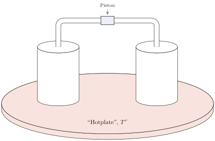
\[ P^{(1)}\left(T^{r}, V^{(1)}, N_{1}^{(1)}, N_{2}^{(1)}, \ldots\right)=P^{(2)}\left(T^{r}, V^{(2)}, N_{1}^{(2)}, N_{2}^{(2)}, \ldots\right) \]
This is one equation involving the two variables \(V^{(1)}\) and \(V^{(2)}\); all other arguments are constant. The closure condition
\[ V^{(1)}+V^{(2)}=V \text {, a constant } \]
provides the other required equation, permitting explicit solution for \(V^{(1)}\) and \(V^{(2)}\).
In the energy representation we would also have found equality of the pressures, as in equation 6.23, but the pressures would be functions of the entropies, volumes, and mole numbers. We would then require the equations of state to relate the entropies to the temperature and the volumes; the two simultaneous equations, 6.23 and 6.24, would be replaced by four.
Although this reduction of four equations to two may seem to be a modest achievement, such a reduction is a very great convenience in more complex situations. Perhaps of even greater conceptual value is the fact that the Helmholtz representation permits us to focus our thought processes exclusively on the subsystem of interest, relegating the reservoir only to an implicit role. And finally, for technical mathematical reasons to be elaborated in Chapter 16, statistical mechanical calculations are enormously simpler in Helmholtz representations, permitting calculations that would otherwise be totally intractable.
For a system in contact with a thermal reservoir the Helmholtz potential can be interpreted as the available work at constant temperature.
Consider a system that interacts with a reversible work source while being in thermal contact with a thermal reservoir. In a reversible process the work input to the reversible work source is equal to the decrease in energy of the system and the reservoir
\[ \begin{aligned} d W_{\mathrm{RWS}} & =-d U-d U^{r}=-d U-T^{r} d S^{r} \\ & =-d U+T^{r} d S=-d\left(U-T^{r} S\right) \\ & =-d F \end{aligned} \]
Thus the work delivered in a reversible process, by a system in contact with a thermal reservoir, is equal to the decrease in the Helmholtz potential of the system. The Helmholtz potential is often referred to as the Helmholtz “free energy,” though the term available work at constant temperature would be less subject to misinterpretation.
Example 1
A cylinder contains an internal piston on each side of which is one mole of a monatomic ideal gas. The walls of the cylinder are diathermal, and the system is immersed in a large bath of liquid (a heat reservoir) at temperature 0°C. The initial volumes of the two gaseous subsystems (on either side of the piston) are 10 liters and 1 liter, respectively. The piston is now moved reversibly, so that the final volumes are 6 liters and 5 liters, respectively. How much work is delivered?
Solution
As the reader has shown in Problem 5.3-1, the fundamental equation of a monatomic ideal gas in the Helmholtz potential representation is
\[ F=N R T\left\{\frac{F_{0}}{N_{0} R T_{0}}-\ln \left[\left(\frac{T}{T_{0}}\right)^{3 / 2} \frac{V}{V_{0}}\left(\frac{N}{N_{0}}\right)^{-1}\right]\right\} \]
At constant \(T\) and \(N\) this is simply
\[ F=\text { constant }-N R T \ln V \]
The change in Helmholtz potential is
\[ \Delta F=-N R T[\ln 6+\ln 5-\ln 10-\ln 1]=-N R T \ln 3=-2.5 \mathrm{~kJ} \]
Thus 2.5 kJ of work are delivered in this process. It is interesting to note that all of the energy comes from the thermal reservoir. The energy of a monatomic ideal gas is simply \(\frac{3}{2} N R T\) and therefore it is constant at constant temperature. The fact that we withdraw heat from the temperature reservoir and deliver it entirely as work to the reversible work source does not, however, violate the Carnot efficiency principle because the gaseous subsystems are not left in their initial state. Despite the fact that the energy of these subsystems remains constant, their entropy increases.
PROBLEMS
Problem 6.2-1
Calculate the pressure on each side of the internal piston in Example 1, for arbitrary position of the piston. By integration then calculate the work done in Example 1 and corroborate the result there obtained.
Problem 6.2-2
Two ideal van der Waals fluids are contained in a cylinder, separated by an internal moveable piston. There is one mole of each fluid, and the two fluids have the same values of the van der Waals constants \(b\) and \(c\); the respective values of the van der Waals constant ” \(a\) ” are \(a_{1}\) and \(a_{2}\). The entire system is in contact with a thermal reservoir of temperature \(T\). Calculate the Helmholtz potential of the composite system as a function of \(T\) and of the total volume \(V\). If the total volume is doubled (while allowing the internal piston to adjust), what is the work done by the system? Recall Problem 5.3-2.
Problem 6.2-3
Two subsystems are contained within a cylinder and are separated by an internal piston. Each subsystem is a mixture of one mole of helium gas and one mole of neon gas (each to be considered as a monatomic ideal gas). The piston is in the center of the cylinder, each subsystem occupying a volume of 10 liters. The walls of the cylinder are diathermal, and the system is in contact with a thermal reservoir at a temperature of \(100^{\circ} \mathrm{C}\). The piston is permeable to helium but impermeable to neon.
Recalling (from Problem 5.3-10) that the Helmholtz potential of a mixture of simple ideal gases is the sum of the individual Helmholtz potentials (each expressed as a function of temperature and volume), show that in the present case
\[ \begin{aligned} F= & N \frac{T}{T_{0}} f_{0}-\frac{3}{2} N R T \ln \frac{T}{T_{0}}-N_{1} R T \ln \left(\frac{V}{V_{0}} \frac{N_{0}}{N_{1}}\right) \\ & -N_{2}^{(1)} R T \ln \frac{V^{(1)} N_{0}}{V_{0} N_{2}^{(1)}}-N_{2}^{(2)} R T \ln \frac{V^{(2)} N_{0}}{V_{0} N_{2}^{(2)}} \end{aligned} \]
where \(T_{0}, f_{0}, V_{0}\), and \(N_{0}\) are attributes of a standard state (recall Problem 5.3-1), \(N\) is the total mole number, \(N_{2}^{(1)}\) is the mole number of neon (component 2) in subsystem 1, and \(V^{(1)}\) and \(V^{(2)}\) are the volumes of subsystems 1 and 2, respectively.
How much work is required to push the piston to such a position that the volumes of the subsystems are 5 liters and 15 liters? Carry out the calculation both by calculating the change in \(F\) and by a direct integration (as in Problem 6.2-1).
Answer:
\[ \text { work }=R T \ln \left(\frac{4}{3}\right)=893 \mathrm{~J} \]
6-3 THE ENTHALPY: THE JOULE-THOMSON OR “THROTTLING” PROCESS
For a composite system in interaction with a pressure reservoir the equilibrium state minimizes the enthalpy over the manifold of states of constant pressure. The enthalpy representation would be appropriate to processes carried out in adiabatically insulated cylinders fitted with adiabatically insulated pistons subject externally to atmospheric pressure, but this is not a very common experimental design. In processes carried out in open vessels, such as in the exercises commonly performed in an elementary chemistry laboratory, the ambient atmosphere acts as a pressure reservoir, but it also acts as a thermal reservoir: for the analysis of such processes only the Gibbs representation invokes the full power of Legendre transformations. Nevertheless, there are particular situations uniquely adapted to the enthalpy representation, as we shall see shortly.
More immediately evident is the interpretation of the enthalpy as a “potential for heat.” From the differential form
\[ d H=T d S+V d P+\mu_{1} d N_{1}+\mu_{2} d N_{2}+\cdots \]
it is evident that for a system in contact with a pressure reservoir and enclosed by impermeable walls
\[ d H=d Q \quad\left(\text { where } P, N_{1}, N_{2}, \ldots \text { are constant }\right) \]
That is, heat added to a system at constant pressure and at constant values of all the remaining extensive parameters (other than \(S\) and \(V\) ) appears as an increase in the enthalpy.
This statement may be compared to an analogous relation for the energy
\[ d U=d Q \quad\left(\text { where } V, N_{1}, N_{2}, \ldots \text { are constant }\right) \]
and similar results for any Legendre transform in which the entropy is not among the transformed variables.
Because heating of a system is so frequently done while the system is maintained at constant pressure by the ambient atmosphere, the enthalpy is generally useful in discussion of heat transfers. The enthalpy accordingly is sometimes referred to as the “heat content” of the system (but it should be stressed again that “heat” refers to a mode of energy flux rather than to an attribute of a state of a thermodynamic system).
To illustrate the significance of the enthalpy as a “potential for heat,” suppose that a system is to be maintained at constant pressure and its volume is to be changed from \(V_{i}\) to \(V_{f}\). We desire to compute the heat absorbed by the system. As the pressure is constant, the heat flux is equal to the change in the enthalpy
\[ Q_{t \rightarrow f} \equiv \int d Q=H_{f}-H_{t} \]
If we were to know the fundamental equation
\[ H=H(S, P, N) \]
then, by differentiation
\[ V=\frac{\partial H}{\partial P}=V(S, P, N) \]
and we could eliminate the entropy to find \(H\) as a function of \(V, P\), and \(N\). Then
\[ Q_{i \rightarrow f}=H\left(V_{f}, P, N\right)-H\left(V_{i}, P, N\right) \]
A process of great practical importance, for which an enthalpy representation is extremely convenient, is the Joule-Thomson or “throttling” process. This process is commonly used to cool and liquify gases and as a second-stage refrigerator in “cryogenic” (low-temperature) laboratories.
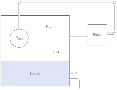
In the Joule-Thomson process or “Joule-Kelvin” process (William Thomson was only later granted peerage as Lord Kelvin) a gas is allowed to seep through a porous barrier from a region of high pressure to a region of low pressure (Fig. 6.2). The porous barrier or “throttling valve” was originally a wad of cotton tamped into a pipe; in a laboratory demonstration it is now more apt to be glass fibers, and in industrial practice it is generally a porous ceramic termination to a pipe (Fig. 6.3). The process can be made continuous by using a mechanical pump to return the gas from the region of low pressure to the region of high pressure. Depending on certain conditions, to be developed in a moment, the gas is either heated or cooled in passing through the throttling valve.
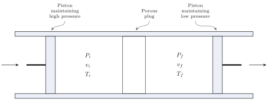
For real gases and for given initial and final pressures, the change in temperature is generally positive down to a particular temperature, and it is negative below that temperature. The temperature at which the process changes from a heating to a cooling process is called the inversion temperature; it depends upon the particular gas and upon both the initial and final pressures. In order that the throttling process operate as an effective cooling process the gas must first be precooled below its inversion temperature.
To show that the Joule-Thomson process occurs at constant enthalpy consider one mole of the gas undergoing a throttling process. The piston
(Fig. 6.2) that pushes this quantity of gas through the plug does an amount of work \(P_{i} v_{i}\), in which \(v_{i}\) is the molar volume of the gas on the high pressure side of the plug. As the gas emerges from the plug, it does work on the piston that maintains the low pressure \(P_{f}\), and this amount of work is \(P_{f} v_{f}\). Thus the conservation of energy determines the final molar energy of the gas; it is the initial molar energy, plus the work \(P_{i} v_{i}\) done on the gas, minus the work \(P_{f} v_{f}\) done by the gas.
\[ u_{f}=u_{i}+P_{i} v_{i}-P_{f} v_{f} \]
or
\[ u_{f}+P_{f} v_{f}=u_{i}+P_{i} v_{i} \]
which can be written in terms of the molar enthalpy \(h\) as
\[ h_{f}=h_{i} \]
Although, on the basis of equation 6.37, we say that the Joule-Thomson process occurs at constant enthalpy, we stress that this simply implies that the final enthalpy is equal to the initial enthalpy. We do not imply anything about the enthalpy during the process; the intermediate states of the gas are nonequilibrium states for which the enthalpy is not defined.
The isenthalpic curves (“isenthalps”) of nitrogen are shown in Fig. 6.4 The initial temperature and pressure in a throttling process determine a particular isenthalp. The final pressure then determines a point on this same isenthalp, thereby determining the final temperature.
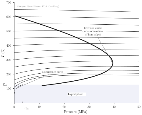
The isenthalps in Fig. 6.4 are concave, with maxima. If the initial temperature and pressure lie to the left of the maximum the throttling process necessarily cools the gas. If the initial temperature lies to the right of the maximum a small pressure drop heats the gas (though a large pressure drop may cross the maximum and can either heat or cool the gas). The maximum of the isenthalp therefore determines the inversion temperature, at which a small pressure change neither heats nor cools the gas.
The dark curve in Fig. 6.4 is a plot of inversion temperature as a function of pressure, obtained by connecting the maxima of the isenthalpic curves. Also shown on the figure is the curve of liquid-gas equilibrium. Points below the curve are in the liquid phase and those above are in the gaseous phase. This coexistence curve terminates in the “critical point.” In the region of this point the “gas” and the “liquid” phases lose their distinguishability, as we shall study in some detail in Chapter 9.
If the change in pressure in a throttling process is sufficiently small we can employ the usual differential analysis.
\[ d T=\left(\frac{\partial T}{\partial P}\right)_{H, N_{1}, N_{2}, \ldots} d P \]
The derivative can be expressed in terms of standard measurable quantities \(\left(c_{p}, \alpha, \kappa_{T}\right)\) by a procedure that may appear somewhat complicated on first reading, but that will be shown in Chapter 7 to follow a routine and straightforward recipe. By a now familiar mathematical identity (A.22),
\[ d T=-\left[\left(\frac{\partial H}{\partial P}\right)_{T} /\left(\frac{\partial H}{\partial T}\right)_{P}\right] d P \]
where we suppress the subscripts \(N_{1}, N_{2}, \ldots\) for simplicity, noting that the mole numbers remain constant throughout. However, \(d H=T d S+V d P\) at constant mole numbers, so that
\[ d T=-\frac{T(\partial S / \partial P)_{T}+V}{T(\partial S / \partial T)_{P}} d P \]
The denominator is \(N c_{P}\). The derivative \((\partial S / \partial P)_{T}\) is equal to \(-(\partial V / \partial T)_{P}\) by one of the class of “Maxwell relations,” analogous to equations 3.62 or 3.65 (in the present case the two derivatives can be corroborated to be the two mixed second derivatives of the Gibbs potential). Identifying \((\partial S / \partial P)_{T}=-(\partial V / \partial T)_{P}=-V \alpha\) (equation 3.67) we finally find
\[ d T=\frac{v}{c_{P}}(T \alpha-1) d P \]
This is a fundamental equation of the Joule-Thomson effect. As the change in pressure \(d P\) is negative, the sign of \(d T\) is opposite that of the quantity in parentheses. Thus if \(T \alpha>1\), a small decrease in pressure (in transiting the “throttling valve”) cools the gas. The inversion temperature is determined by
\[ \alpha T_{\text {inversion }}=1 \]
For an ideal gas the coefficient of thermal expansion \(\alpha\) is equal to \(1 / T\), so that there is no change in temperature in a Joule-Thomson expansion. All gases approach ideal behavior at high temperature and low or moderate pressure, and the isenthalps correspondingly become “flat,” as seen in Fig. 6.4. It is left to Example 2 to show that for real gases the temperature change is negative below the inversion temperature and positive above, and to evaluate the inversion temperature.
Example 2
Compute the inversion temperature of common gases, assuming them to be described by the van der Waals equation of state (3.41).
Solution We must first evaluate the coefficient of expansion \(\alpha\). Differentiating the van der Waals equation of state (3.41) with respect to \(T\), at constant \(P\)
\[ \alpha=\frac{1}{v}\left(\frac{\partial v}{\partial T}\right)_{P}=\left[\frac{T v}{v-b}-\frac{2 a(v-b)}{R v^{2}}\right]^{-1} \]
To express the right-hand side as a function of \(T\) and \(P\) is analytically difficult. An approximate solution follows from the recognition that molar volumes are on the order of \(0.02 \mathrm{~m}^{3}\), whence \(\mathrm{b} / v\) is on the order of \(10^{-3}\) and \(a / \mathrm{RT} v\) is on the order of \(10^{-3}-10^{-4}\) (see Table 3.1). Hence a series expansion in \(\mathrm{b} / \mathrm{v}\) and \(a / \mathrm{RT} v\) can reasonably be terminated at the lowest order term. Let
\[ \varepsilon_{1} \equiv \frac{b}{v} \quad \varepsilon_{2} \equiv \frac{a}{\mathrm{RT} v} \]
Then
\[ \begin{aligned} \alpha & =\left[\frac{T}{1-\varepsilon_{1}}-\frac{2 T}{v}(v-b) \varepsilon_{2}\right]^{-1} \\ & =\frac{1}{T}\left[\frac{1}{1-\varepsilon_{1}}-2\left(1-\varepsilon_{1}\right) \varepsilon_{2}\right]^{-1} \end{aligned} \]
Returning to equation 6.41 from which we recall that
\[ d T=\frac{v}{c_{p}}(T \alpha-1) d P \]
\[ T_{\text {inv }} \alpha=1 \]
It then follows that at the inversion temperature
\[ \left[1-\varepsilon_{1}+2 \varepsilon_{2}+\cdots\right]=1 \]
or
\[ \varepsilon_{1}=2 \varepsilon_{2} \]
The inversion temperature is now determined by
\[ T_{\mathrm{inv}} \simeq \frac{2 a}{b R} \]
with cooling of the gas for temperature below \(T_{\text {inv }}\), and heating above. From Table 3.1, we compute the inversion temperature of several gases: \(T_{\text {inv }}\left(\mathrm{H}_{2}\right)=224\) \(\mathrm{K}, T_{\text {inv }}(\mathrm{Ne})=302 \mathrm{~K}, T_{\text {inv }}\left(\mathrm{N}_{2}\right)=850 \mathrm{~K}, T_{\text {inv }}\left(\mathrm{O}_{2}\right)=1020 \mathrm{~K}, T_{\text {inv }}\left(\mathrm{CO}_{2}\right)=2260\) K. In fact the inversion temperature empirically depends strongly on the pressure -a dependence lost in our calculation by the neglect of higher-order terms. The observed inversion temperature at zero pressure for \(\mathrm{H}_{2}\) is 204 K, and for neon it is 228 K-in fair agreement with our crude calculation. For polyatomic gases the agreement is less satisfactory; the observed value for \(\mathrm{CO}_{2}\) is 1275 K whereas we have computed 2260 K.
PROBLEMS
Problem 6.3-1
A hole is opened in the wall separating two chemically identical singlecomponent subsystems. Each of the subsystems is also in interaction with a
pressure reservoir of pressure \(P^{r}\). Use the enthalpy minimum principle to show that the conditions of equilibrium are \(T^{(1)}=T^{(2)}\) and \(\mu^{(1)}=\mu^{(2)}\).
Problem 6.3-2
A gas has the following equations of state
\[ P=\frac{U}{V} \quad T=3 B\left(\frac{U^{2}}{N V}\right)^{1 / 3} \]
where \(B\) is a positive constant. The system obeys the Nernst postulate ( \(S \rightarrow 0\) as \(T \rightarrow 0\) ). The gas, at an initial teperature \(T_{1}\) and initial pressure \(P_{t}\), is passed through a “porous plug” in a Joule-Thomson process. The final pressure is \(P_{f}\).Calculate the final temperature \(T_{f}\).
Problem 6.3-3
Show that for an ideal van der Waals fluid
\[ h=-\frac{2 a}{v}+R T\left(c+\frac{v}{v-b}\right) \]
where \(h\) is the molar enthalpy. Assuming such a fluid to be passed through a porous plug and thereby expanded from \(v_{i}\) to \(v_{f}\) (with \(v_{f}>v_{i}\) ), find the final temperature \(T_{f}\) in terms of the initial temperature \(T_{i}\) and the given data.
Evaluate the temperature change if the gas is \(\mathrm{CO}_{2}\), the mean temperature is \(0^{\circ} \mathrm{C}\), the mean pressure is \(10^{7} \mathrm{~Pa}\), and the change in pressure is \(10^{6} \mathrm{~Pa}\). The molar heat capacity \(c_{P}\) of \(\mathrm{CO}_{2}\) at the relevant temperature and pressure is 29.5 J/mole-K. Carry calculation only to first order in \(b / v\) and \(a / \mathrm{RT} v\).
Problem 6.3-4
One mole of a monatomic ideal gas is in a cylinder with a movable piston on the other side of which is a pressure reservoir with \(P_{r}=1 \mathrm{~atm}\). How much heat must be added to the gas to increase its volume from 20 to 50 liters?
Problem 6.3-5
Assume that the gas of Problem 6.3-4 is an ideal van der Waals fluid with the van der Waals constants of argon (Table 3-1), and again calculate the heat required. Recall Problem 6.3-3.
6-4 THE GIBBS POTENTIAL; CHEMICAL REACTIONS
For a composite system in interaction with both thermal and pressure reservoirs the equilibrium state minimizes the Gibbs potential over the manifold of states of constant temperature and pressure (equal to those of the reservoirs).
The Gibbs potential is a natural function of the variables \(T, P, N_{1}, N_{2}, \ldots\), and it is particularly convenient to use in the analysis of problems involving constant \(T\) and \(P\). Innumerable processes of common experience occur in systems exposed to the atmosphere, and thereby maintained at constant temperature and pressure. And frequently a process of interest occurs in a small subsystem of a larger system that acts as both a thermal and a pressure reservoir (as in the fermentation of a grape in a large wine vat).
The Gibbs potential of a multicomponent system is related to the chemical potentials of the individual components, for \(G=U-T S+P V\), and inserting the Euler relation \(U=T S-P V+\mu_{1} N_{1}+\mu_{2} N_{2}+\cdots\) we find
\[ G=\mu_{1} N_{1}+\mu_{2} N_{2}+\cdots \]
Thus, for a single component system the molar Gibbs potential is identical with \(\mu\)
\[ \frac{G}{N}=\mu \]
but for a multicomponent system
\[ \frac{G}{N}=\mu_{1} x_{1}+\mu_{2} x_{2}+\cdots+\mu_{r} x_{r} \]
where \(x_{j}\) is the mole fraction \(\left(N_{j} / N\right)\) of the \(j\) th component. Accordingly, the chemical potential is often referred to as the molar Gibbs potential in single component systems or as the partial molar Gibbs potential in multicomponent systems.
The thermodynamics of chemical reactions is a particularly important application of the Gibbs potential.
Consider the chemical reaction
\[ 0 \rightleftarrows \sum_{1}^{r} \nu_{j} A_{j} \]
where the \(\nu\) are the stoichiometric coefficients defined in Section 2.9. The change in Gibbs potential associated with virtual changes \(d N_{j}\) in the mole numbers is
\[ d G=-S d T+V d P+\sum_{j} \mu_{j} d N_{j} \]
However the changes in the mole numbers must be in proportion to the stoichiometric coefficients, so that
\[ \frac{d N_{1}}{\nu_{1}}=\frac{d N_{2}}{\nu_{2}}=\cdots \equiv d \tilde{N} \]
or, equivalently,
\[ d N_{j}=\nu_{j} d \tilde{N} \]
where \(d \tilde{N}\) is simply a proportionality factor defined by equation 6.48. If the chemical reaction is carried out at constant temperature and pressure (as in an open vessel) the condition of equilibrium then implies
\[ d G=d \tilde{N} \sum_{j} \nu_{j} \mu_{j}=0 \]
or
\[ \sum_{j} \nu_{j} \mu_{j}=0 \]
If the initial quantities of each of the chemical components is \(N_{j}^{0}\) the chemical reaction proceeds to some extent and the mole numbers assume the new values
\[ N_{j}=N_{j}^{0}+\int d N_{j}=N_{j}^{0}+\nu_{j} \Delta \tilde{N} \]
where \(\Delta \tilde{N}\) is the factor of proportionality. The chemical potentials in equation 6.51 are functions of \(T, P\), and the mole numbers, and hence of the single unknown parameter \(\Delta \tilde{N}\). Solution of equation 6.51 for \(\Delta \tilde{N}\) determines the equilibrium composition of the system.
The solution described is appropriate only providing that there is a sufficient quantity of each component present so that none is depleted before equilibrium is reached. That is, none of the quantities \(N_{j}\) in equation 6.52 can become negative. This consideration is most conveniently expressed in terms of the degree of reaction.
The maximum value of \(\Delta \tilde{N}\) for which all \(N_{j}\) remain positive (in equation 6.52) defines the maximum permissible extent of the reaction. Similarly the minimum value of \(\Delta \tilde{N}\) for which all \(N_{j}\) remain positive defines the maximum permissible extent of the reverse reaction. The actual value of \(\Delta \tilde{N}\) in equilibrium may be anywhere between these two extremes. The degree of reaction \(\varepsilon\) is defined as
\[ \varepsilon \equiv \frac{\Delta \tilde{N}-\Delta \tilde{N}_{\mathrm{min}}}{\Delta \tilde{N}_{\mathrm{max}}-\Delta \tilde{N}_{\mathrm{min}}} \]
It is possible that a straightforward solution of the equation of chemical equilibrium (6.51) may yield a value of \(\Delta \tilde{N}\) that is larger than \(\Delta \tilde{N}_{\max }\) or smaller than \(\Delta \tilde{N}_{\text {min }}\). In such a case the process is terminated by the depletion of one of its components. The physically relevant value of \(\Delta \tilde{N}\) is then \(\Delta \tilde{N}_{\text {max }}\) (or \(\Delta \tilde{N}_{\text {min }}\) ). Although \(\sum_{j} \nu_{j} \mu_{j}\) does not attain the value zero, it does attain the smallest absolute value accessible to the system.
Whereas the partial molar Gibbs potentials characterize the equilibrium condition, the enthalpy finds its expression in the heat of reaction. This fact follows from the general significance of the enthalpy as a “potential for heat flux” at constant pressure (equation 6.29). That is, the flux of heat from the surroundings to the system, during the chemical reaction, is equal to the change in the enthalpy. This change in enthalpy, in turn, can be related to the chemical potentials, for
\[ H=G+T S=G-T\left(\frac{\partial G}{\partial T}\right)_{P, N_{1}, N_{2}, \ldots} \]
If an infinitesimal chemical reaction \(d \tilde{N}\) occurs, both \(H\) and \(G\) change and
\[ d H=\frac{d H}{d \tilde{N}} d \tilde{N}=\frac{d G}{d \tilde{N}} d \tilde{N}-T \frac{\partial}{\partial T}\left(\frac{d G}{d \tilde{N}}\right)_{P, N_{1}, N_{2},} d \tilde{N} \]
But the change in Gibbs function is
\[ d G=\sum_{1}^{r} \mu_{j} d N_{j}=\left(\sum_{1}^{r} \nu_{j} \mu_{j}\right) d \tilde{N} \]
whence
\[ \frac{d G}{d \tilde{N}}=\sum_{1}^{r} \nu_{j} \mu_{j} \]
At equilibrium \(d G / d \tilde{N}\) vanishes (but the temperature derivative of \(d G / d \tilde{N}\) does not) so that in the vicinity of the equilibrium state equation 6.55 becomes
\[ \frac{d H}{d \tilde{N}}=-T \frac{\partial}{\partial T}\left(\sum_{1}^{r} \nu_{j} \mu_{j}\right)_{P, N_{1}, N_{2}, \ldots} \]
The quantity \(d H / d \tilde{N}\) is known as the heat of reaction; it is the heat absorbed per unit reaction in the vicinity of the equilibrium state. It is positive for endothermic reactions and negative for exothermic reactions.
We have assumed that the reaction considered is not one that goes to completion. If the reaction does go to completion, the summation in equation 6.57 does not vanish in the equilibrium state, and this summation appears as an additional term in equation 6.58.
As the summation in equation 6.58 vanishes at the equilibrium composition, it is intuitively evident that the temperature derivative of this quantity is related to the temperature dependence of the equilibrium concentrations. We shall find it convenient to develop this connection explicitly only in the special case of ideal gases, in Section 13.4. However, it is of interest here to note the plausibility of the relationship and to recognize that such a relationship permits the heat of reaction to be measured by determinations of equilibrium compositions at various temperatures rather than by relatively difficult calorimetric experiments.
The general methodology for the analysis of chemical reactions becomes specific and definite when applied to particular systems. To anchor the foregoing treatment in a fully explicit (and practically important) special case, the reader may well wish here to interpolate Chapter 13-and particularly Section 13.2 on chemical reactions in ideal gases.
Example 3
Five moles of \(\mathrm{H}_{2}, 1\) mole of \(\mathrm{CO}_{2}, 1\) mole of \(\mathrm{CH}_{4}\), and 3 moles of \(\mathrm{H}_{2} \mathrm{O}\) are allowed to react in a vessel maintained at a temperature \(T_{0}\) and pressure \(P_{0}\). The relevant reaction is
\[ 4 \mathrm{H}_{2}+\mathrm{CO}_{2} \rightleftharpoons \mathrm{CH}_{4}+2 \mathrm{H}_{2} \mathrm{O} \]
Solution of the equilibrium condition gives the nominal solution \(\Delta \tilde{N}=-\frac{1}{2}\). What are the mole numbers of each of the components? If the pressure is then increased to \(P_{1}\left(P_{1}>P_{0}\right)\) and the temperature is maintained constant \(\left(=T_{0}\right)\) the equilibrium condition gives a new nominal solution of \(\Delta \tilde{N}=1,2\). What are the mole numbers of each of the components?
Solution
We first write the analogue of equation 6.52 for each component: \(N_{\mathrm{H}_{2}}=\) \(5-4 \Delta \tilde{N}, N_{\mathrm{CO}_{2}}=1-\Delta \tilde{N}, N_{\mathrm{CH}_{4}}=1+\Delta \tilde{N}, N_{\mathrm{H}_{2} \mathrm{O}}=3+2 \Delta \tilde{N}\). Setting each of these mole numbers equal to zero successively we find four roots for \(\Delta \tilde{N}: \frac{5}{4}, 1\), -1 , and \(-\frac{3}{2}\). The positive and negative roots of smallest absolute values are, respectively,
\[ \Delta \tilde{N}_{\max }=1 \quad \Delta \tilde{N}_{\min }=-1 \]
These two bounds on \(\Delta \tilde{N}\) correspond to depletion of \(\mathrm{CO}_{2}\) if the reaction proceeds too far in the “forward” direction, and to depletion of \(\mathrm{CH}_{4}\) if the reaction proceeds too far in the “reverse” direction.
The degree of reaction is now, by equation 6.53
\[ \varepsilon=\frac{\Delta \tilde{N}+1}{1+1}=\frac{1}{2}(\Delta \tilde{N}+1) \]
If the nominal solution of the equilibrium condition gives \(\Delta \tilde{N}=-\frac{1}{2}\) then \(\varepsilon=\frac{1}{4}\) and \(N_{\mathrm{H}_{2}}=3, N_{\mathrm{CO}_{2}}=\frac{3}{2}, N_{\mathrm{CH}_{4}}=\frac{1}{2}\) and \(N_{\mathrm{H}_{2} \mathrm{O}}=2\).
If the increase in pressure shifts the nominal solution for \(\Delta \bar{N}\) to \(+1,2\) we reject this value as outside the acceptable range of \(\Delta \bar{N}\) (i.e., greater than \(\Delta \bar{N}_{\text {max }}\) ); it would lead to the nonphysical value of \(\varepsilon=1.1\) whereas \(\varepsilon\) must be between zero and unity. Hence the reaction is terminated at \(\Delta \bar{N}=\Delta \bar{N}_{\text {max }}=\frac{1}{2}\) (or at \(\varepsilon=1\) ) by the depletion of \(\mathrm{CO}_{2}\). The final mole numbers are \(N_{\mathrm{H}_{2}}=1, N_{\mathrm{CO}_{2}}=\frac{1}{2}, N_{\mathrm{CH}_{4}}=2\), and \(N_{\mathrm{H}_{2} \mathrm{O}}=5\).
PROBLEMS
Problem 6.4-1
One half mole of \(\mathrm{H}_{2} \mathrm{~S}, \frac{3}{4}\) mole of \(\mathrm{H}_{2} \mathrm{O}, 2\) moles of \(\mathrm{H}_{2}\), and 1 mole of \(\mathrm{SO}_{2}\) are allowed to react in a vessel maintained at a temperature of 300 K and a pressure of \(10^{4} \mathrm{~Pa}\). The components can react by the chemical reaction
\[ 3 \mathrm{H}_{2}+\mathrm{SO}_{2} \rightleftharpoons \mathrm{H}_{2} \mathrm{~S}+2 \mathrm{H}_{2} \mathrm{O} \]
Write the condition of equilibrium in terms of the partial molar Gibbs potentials.
Show that
\[ N_{\mathrm{H}_{2}}=2-3 \Delta \tilde{N} \]
and similarly for the other components. For what value of \(\Delta \tilde{N}\) does each \(N_{j}\) vanish?
Show that \(\Delta \tilde{N}_{\text {max }}=\frac{2}{3}\) and \(\Delta \tilde{N}_{\text {min }}=-\frac{3}{8}\). Which components are depleted in each of these cases?
Assume that the nominal solution of the equilibrium condition gives \(\Delta \tilde{N}=\frac{1}{4}\). What is the degree of reaction \(\varepsilon\) ? What are the mole fractions of each of the components in the equilibrium mixture?
Assume that the pressure is raised and that the nominal solution of the equilibrium condition now yields the value \(\Delta \tilde{N}=0.8\). What is the degree of reaction? What are the mole fractions of each of the components in the final state?
Answers:
- \(\mathrm{H}_{2}\) and \(\mathrm{H}_{2} \mathrm{O}\) depleted
\[ \varepsilon=\frac{3}{5}, \]
\[ x_{\mathrm{H}_{2} \mathrm{O}}=\frac{5}{16} \]
\[ \Delta \tilde{N}=\frac{2}{3}, \]
\[ x_{\mathrm{H}_{2} \mathrm{O}}=.59 \]
6-5 OTHER POTENTIALS
Various other potentials may occasionally become useful in particular applications. One such application will suffice to illustrate the general method.
Example 4
A bottle, of volume \(V\), contains \(N_{s}\) moles of sugar, and it is filled with water and capped by a rigid lid. The lid though rigid is permeable to water but not to sugar. The bottle is immersed in a large vat of water. The pressure in the vat, at the position of the bottle, is \(P_{v}\) and the temperature is \(T\). We seek the pressure \(P\) and the mole number \(N_{w}\) of water in the bottle. Solution We suppose that we are given the fundamental equation of a two-component mixture of sugar and water. Most conveniently, this fundamental equation will be cast in the representation \(U\left[T, V, \mu_{w,} N_{s}\right]\); that is, in the representation in which \(S\) and \(N_{w}\) are replaced by their corresponding intensive parameters, but the volume \(V\) and the mole number of sugar \(N_{s}\) remain untransformed. The diathermal wall ensures that \(T\) has the value established by the vat (a thermal reservoir), and the semipermeable lid ensures that \(\mu_{w}\) has the value established by the vat (a “water reservoir”). No problem remains! We know all the independent variables of the generalized potential \(U\left[T, V, \mu_{w}, N_{s}\right]\). To find the pressure in the bottle we merely differentiate the potential:
\[ P=-\frac{\partial U\left[T, V, \mu_{w}, N_{s}\right]}{\partial V} \]
It is left to the reader to compare this approach to the solution of the same problem in energy or entropy representations. Various unsought for variables enter into the analysis-such as the entropy of the contents of the bottle, or the entropy, energy, and mole number of the contents of the vat. And for each such extraneous variable, an additional equation is needed for its elimination. The choice of the appropriate representation clearly is the key to simplicity, and indeed to practicality, in thermodynamic calculations.
6-6 COMPILATIONS OF EMPIRICAL DATA; THE ENTHALPY OF FORMATION
In principle, thermodynamic data on specific systems would be most succinctly and conveniently given by a tabulation of the Gibbs potential as a function of temperature, pressure, and composition (mole fractions of the individual components). Such a tabulation would provide a fundamental equation in the representation most convenient to the experimentalist.
In practice it is customary to compile data on \(h(T, P), s(T, P)\), and \(v(T, P)\), from which the molar Gibbs potential can be obtained ( \(g=h-\) \(T s\) ). The tabulation of \(h, s\), and \(v\) is redundant but convenient. For multicomponent systems analogous compilations must be made for each composition of interest.
Differences in the molar enthalpies of two states of a system can be evaluated experimentally by numerical integration of \(d h=d Q / N+v d P\), for \(d Q\) as well as \(P\) and \(v\) can be measured along the path of integration.
The absolute scale of the enthalpy \(h\), like that of the energy or of any other thermodynamic potential, is arbitrary, undetermined within an additive constant. For purposes of compilation of data, the scale of enthalpy is made definite by assigning the value zero to the molar enthalpy of each chemical element in its most stable form at a standard temperature and pressure, generally taken as
\[ T_{0}=298.15 \mathrm{~K}=25^{\circ} \mathrm{C} \quad P_{0}=0.1 \mathrm{MPa} \approx 1 \mathrm{~atm} \]
The enthalpy defined by this choice of scale is called the enthalpy of formation.
The reference to the “most stable state” in the definition of the enthalpy of formation implies, for instance, that the value zero is assigned to the molecular form of oxygen \(\left(\mathrm{O}_{2}\right)\) rather than to the atomic form \((\mathrm{O})\); the molecular form is the most stable form at standard temperature and pressure.
If 1 mole of carbon and 1 mole of \(\mathrm{O}_{2}\) are chemically reacted to form 1 mole of \(\mathrm{CO}_{2}\), the reaction being carried out at standard temperature and pressure, it is observed that \(393.52 \times 10^{3} \mathrm{~J}\) of heat are emitted. Hence the enthalpy of formation of \(\mathrm{CO}_{2}\) is taken as \(-393.52 \times 10^{3} \mathrm{~J} /\) mole in the standard state. This is the standard enthalpy of formation of \(\mathrm{CO}_{2}\). The enthalpy of formation of \(\mathrm{CO}_{2}\) at any other temperature and pressure is obtained by integration of \(d h=d Q / N+v d P\).
The standard molar enthalpy of formation, the corresponding standard molar Gibbs potential, and the molar entropy in the standard state are tabulated for a wide range of compounds in the JANAF Thermochemical Tables (Dow Chemical Company, Midland, Michigan) and in various other similar compilations.
Tables of thermodynamic properties of a particular material can become very voluminous indeed if several properties (such as \(h, s\), and \(v\) ), or even a single property, are to be tabulated over wide ranges of theindependent variables \(T\) and \(P\). Nevertheless, for common materials such as water very extensive tabulations are readily available. In the case of water the tabulations are referred to as “Steam Tables.” One form of steam table, referred to as a “superheated steam table,” gives values of the molar volume \(v\), energy \(u\), enthalpy \(h\), and entropy \(s\) as a function of temperature, for various values of pressure. An excerpt from such a table (by Sonntag and van Wilen), for a few values of the pressure, is given in Table 6.1. Another form, referred to as a “saturated steam table,” gives values of the properties of the liquid and of the gaseous phases of water for values of \(P\) and \(T\) which lie on the gas-liquid coexistence curve. Such a “saturated steam table” will be given in Table 9.1. Another very common technique for representation of thermodynamic data consists of “thermodynamic charts,” or graphs. Such charts necessarily sacrifice precision, but they allow a large amount of data to be summarized succinctly and compactly. Conceptually, the simplest such chart would label the two coordinate axes by \(T\) and \(P\). Then, for a single-component system one would draw families of curves of constant molar Gibbs potential \(\mu\). In principle that would permit evaluation of all desired data. Determination of the molar volume, for instance, would require reading the values of \(\mu\) for two nearby pressures at the temperature of interest; this would permit numerical evaluation of the derivative \((\Delta \mu / \Delta P)_{T}\), and thence of the molar volume. Instead, a family of isochores is overlaid on the graph, with each isochore labeled by \(v\). Similarly,
TABLE 6.1 Superheated Steam Table The quantities \(u, h\), and \(s\) are per unit mass (rather than molar); the units of \(u\) and \(h\) are Joules/kilogram, of \(v\) are \(\mathrm{m}^{3} /\) kilogram , and of \(s\) are Joules/kilogram-Kelvin. Temperatures are in degrees Celsius. The notation “Sat.” under \(T\) refers to the temperature on the liquid-gas coexistence curve; this temperature is given in parentheses following each pressure value. From R. E. Sonntag and G. Van Wylen, Introduction to Thermodynamics, Classical and Statistical, John Wiley & Sons, New York, 1982.
| \(T\) | \(P=.010 \mathrm{MPa}(45.81)\) | \(P=.050 \mathrm{MPa}(81.33)\) | \(P=.10 \mathrm{MPa}(99.63)\) | |||||||||
|---|---|---|---|---|---|---|---|---|---|---|---|---|
| \(v\) | \(u\) | \(h\) | \(s\) | \(v\) | \(u\) | \(h\) | \(s\) | \(v\) | \(u\) | \(h\) | \(s\) | |
| Sat. | 14.674 | 2437.9 | 2584.7 | 8.1502 | 3.240 | 2483.9 | 2645.9 | 7.5939 | 1.6940 | 2506.1 | 2675.5 | 7.3594 |
| 50 | 14.869 | 2443.9 | 2592.6 | 8.1749 | ||||||||
| 100 | 17.196 | 2515.5 | 2687.5 | 8.4479 | 3.418 | 2511.6 | 2682.5 | 7.6947 | 1.6958 | 2506.7 | 2676.2 | 7.3614 |
| 150 | 19.512 | 2587.9 | 2783.0 | 8.6882 | 3.889 | 2585.6 | 2780.1 | 7.9401 | 1.9364 | 2582.8 | 2776.4 | 7.6134 |
| 200 | 21.825 | 2661.3 | 2879.5 | 8.9038 | 4.356 | 2659.9 | 2877.7 | 8.1580 | 2.172 | 2658.1 | 2875.3 | 7.8343 |
| 250 | 24.136 | 2736.0 | 2977.3 | 9.1002 | 4.820 | 2735.0 | 2976.0 | 8.3556 | 2.406 | 2733.7 | 2974.3 | 8.0333 |
| 300 | 26.445 | 2812.1 | 3076.5 | 9.2813 | 5.284 | 2811.3 | 3075.5 | 8.5373 | 2.639 | 2810.4 | 3074.3 | 8.2158 |
| 400 | 31.063 | 2968.9 | 3279.6 | 9.6077 | 6.209 | 2968.5 | 3278.9 | 8.8642 | 3.103 | 2967.9 | 3278.2 | 8.5435 |
| 500 | 35.679 | 3132.3 | 3489.1 | 9.8978 | 7.134 | 3132.0 | 3488.7 | 9.1546 | 3.565 | 3131.6 | 3488.1 | 8.8342 |
| 600 | 40.295 | 3302.5 | 3705.4 | 10.1608 | 8.057 | 3302.2 | 3705.1 | 9.4178 | 4.028 | 3301.9 | 3704.7 | 9.0976 |
| 700 | 44.911 | 3479.6 | 3928.7 | 10.4028 | 8.981 | 3479.4 | 3928.5 | 9.6599 | 4.490 | 3479.2 | 3928.2 | 9.3398 |
| 800 | 49.526 | 3663.8 | 4159.0 | 10.6281 | 9.904 | 3663.6 | 4158.9 | 9.8852 | 4.952 | 3663.5 | 4158.6 | 9.5652 |
| 900 | 54.141 | 3855.0 | 4396.4 | 10.8396 | 10.828 | 3854.9 | 4396.3 | 10.0967 | 5.414 | 3854.8 | 4396.1 | 9.7767 |
| 1000 | 58.757 | 4053.0 | 4640.6 | 11.0393 | 11.751 | 4052.9 | 4640.5 | 10.2964 | 5.875 | 4052.8 | 4640.3 | 9.9764 |
| 1100 | 63.372 | 4257.5 | 4891.2 | 11.2287 | 12.674 | 4257.4 | 4891.1 | 10.4859 | 6.337 | 4257.3 | 4891.0 | 10.1659 |
| 1200 | 67.987 | 4467.9 | 5147.8 | 11.4091 | 13.597 | 4467.8 | 5147.7 | 10.6662 | 6.799 | 4467.7 | 5147.6 | 10.3463 |
| 1300 | 72.602 | 4683.7 | 5409.7 | 11.5811 | 14.521 | 4683.6 | 5409.6 | 10.8382 | 7.260 | 4683.5 | 5409.5 | 10.5183 |
| \(P=.20 \mathrm{MPa}(120.23)\) | TABLE 6.1 (Continued) \(P=.30 \mathrm{MPa}\) (133.55) | \(P=.40 \mathrm{MPa}(143.63)\) | ||||||||||
|---|---|---|---|---|---|---|---|---|---|---|---|---|
| Sat. | . 8857 | 2529.5 | 2706.7 | 7.1272 | . 6058 | 2543.6 | 2725.3 | 6.9919 | . 4625 | 2553.6 | 2738.6 | 6.8959 |
| 150 | . 9596 | 2576.9 | 2768.8 | 7.2795 | . 6339 | 2570.8 | 2761.0 | 7.0778 | . 4708 | 2564.5 | 2752.8 | 6.9299 |
| 200 | 1.0803 | 2654.4 | 2870.5 | 7.5066 | . 7163 | 2650.7 | 2865.6 | 7.3115 | . 5342 | 2646.8 | 2860.5 | 7.1706 |
| 250 | 1.1988 | 2731.2 | 2971.0 | 7.7086 | . 7964 | 2728.7 | 2967.6 | 7.5166 | . 5951 | 2726.1 | 2964.2 | 7.3789 |
| 300 | 1.3162 | 2808.6 | 3071.8 | 7.8926 | . 8753 | 2806.7 | 3069.3 | 7.7022 | . 6548 | 2804.8 | 3066.8 | 7.5662 |
| 400 | 1.5493 | 2966.7 | 3276.6 | 8.2218 | 1.0315 | 2965.6 | 3275.0 | 8.0330 | . 7726 | 2964.4 | 3273.4 | 7.8985 |
| 500 | 1.7814 | 3130.8 | 3487.1 | 8.5133 | 1.1867 | 3130.0 | 3486.0 | 8.3251 | . 8893 | 3129.2 | 3484.9 | 8.1913 |
| 600 | 2.013 | 3301.4 | 3704.0 | 8.7770 | 1.3414 | 3300.8 | 3703.2 | 8.5892 | 1.0055 | 3300.2 | 3702.4 | 8.4558 |
| 700 | 2.244 | 3478.8 | 3927.6 | 9.0194 | 1.4957 | 3478.4 | 3927.1 | 8.8319 | 1.1215 | 3477.9 | 3926.5 | 8.6987 |
| 800 | 2.475 | 3663.1 | 4158.2 | 9.2449 | 1.6499 | 3662.9 | 4157.8 | 9.0576 | 1.2372 | 3662.4 | 4157.3 | 8.9244 |
| 900 | 2.706 | 3854.5 | 4395.8 | 9.4566 | 1.8041 | 3854.2 | 4395.4 | 9.2692 | 1.3529 | 3853.9 | 4395.1 | 9.1362 |
| 1000 | 2.937 | 4052.5 | 4640.0 | 9.6563 | 1.9581 | 4052.3 | 4639.7 | 9.4690 | 1.4685 | 4052.0 | 4639.4 | 9.3360 |
| 1100 | 3.168 | 4257.0 | 4890.7 | 9.8458 | 2.1121 | 4256.8 | 4890.4 | 9.6585 | 1.5840 | 4256.5 | 4890.2 | 9.5256 |
| 1200 | 3.399 | 4467.5 | 5147.3 | 10.0262 | 2.2661 | 4467.2 | 5147.1 | 9.8389 | 1.6996 | 4467.0 | 5146.8 | 9.7060 |
| 1300 | 3.630 | 4683.2 | 5409.3 | 10.1982 | 2.4201 | 4683.0 | 5409.0 | 10.0110 | 1.8151 | 4682.8 | 5408.8 | 9.8780 |
| \(P=.50 \mathrm{MPa}(151.86)\) | \(P=.60 \mathrm{MPa}(158.85)\) | \(P=.80 \mathrm{MPa}(170.43)\) | ||||||||||
| Sat. | . 3749 | 2561.2 | 2748.7 | 6.8213 | . 3157 | 2567.4 | 2756.8 | 6.7600 | . 2404 | 2576.8 | 2769.1 | 6.6628 |
| 200 | . 4249 | 2642.9 | 2855.4 | 7.0592 | . 3520 | 2638.9 | 2850.1 | 6.9665 | . 2608 | 2630.6 | 2839.3 | 6.8158 |
| 250 | . 4744 | 2723.5 | 2960.7 | 7.2709 | . 3938 | 2720.9 | 2957.2 | 7.1816 | . 2931 | 2715.5 | 2950.0 | 7.0384 |
| 300 | . 5226 | 2802.9 | 3064.2 | 7.4599 | . 4344 | 2801.0 | 3061.6 | 7.3724 | . 3241 | 2797.2 | 3056.5 | 7.2328 |
| 350 | . 5701 | 2882.6 | 3167.7 | 7.6329 | . 4742 | 2881.2 | 3165.7 | 7.5464 | . 3544 | 2878.2 | 3161.7 | 7.4089 |
| 400 | . 6173 | 2963.2 | 3271.9 | 7.7938 | . 5137 | 2962.1 | 3270.3 | 7.7079 | . 3843 | 2959.7 | 3267.1 | 7.5716 |
| 500 | . 7109 | 3128.4 | 3483.9 | 8.0873 | . 5920 | 3127.6 | 3482.8 | 8.0021 | . 4433 | 3126.0 | 3480.6 | 7.8673 |
| 600 | . 8041 | 3299.6 | 3701.7 | 7.3522 | . 6697 | 3299.1 | 3700.9 | 8.2674 | . 5018 | 3297.9 | 3699.4 | 8.1333 |
| 700 | . 8969 | 3477.5 | 3925.9 | 8.5952 | . 7472 | 3477.0 | 3925.3 | 8.5107 | . 5601 | 3476.2 | 3924.2 | 8.3770 |
| 800 | . 9896 | 3662.1 | 4156.9 | 8.8211 | . 8245 | 3661.8 | 4156.5 | 8.7367 | . 6181 | 3661.1 | 4155.6 | 8.6033 |
| 900 | 1.0822 | 3853.6 | 4394.7 | 9.0329 | . 9017 | 3853.4 | 4394.4 | 8.9486 | . 6761 | 3852.8 | 4393.7 | 8.8153 |
| 1000 | 1.1747 | 4051.8 | 4639.1 | 9.2328 | . 9788 | 4051.5 | 4638.8 | 9.1485 | . 7340 | 4051.0 | 4638.2 | 9.0153 |
| 1100 | 1.2672 | 4256.3 | 4889.9 | 9.4224 | 1.0559 | 4256.1 | 4889.6 | 9.3381 | . 7919 | 4255.6 | 4889.1 | 9.2050 |
| 1200 | 1.3596 | 4466.8 | 5146.6 | 9.6029 | 1.1330 | 4466.5 | 5146.3 | 9.5185 | . 8497 | 4466.1 | 5145.9 | 9.3855 |
| 1300 | 1.4521 | 4682.5 | 5408.6 | 9.7749 | 1.2101 | 4682.3 | 5408.3 | 9.6906 | . 9076 | 4681.8 | 5407.9 | 9.5575 |
families of constant molar entropy \(s\), of constant molar enthalpy \(h\), of constant coefficient of thermal expansion \(\alpha\), of constant \(\kappa_{T}\), and the like are also overlaid. The limit is set by readability of the chart.
It will be recognized that there is nothing unique about the variables assigned to the cartesian axes. Each family of curves serves as a (curvilinear) coordinate system. Thus a point of given \(v\) and \(s\) can be located as the intersection of the corresponding isochore and adiabat, and the value of any other plotted variable can then be read.
In practice there are many variants of thermodynamic charts in use. A popular type of chart is known as a Mollier chart -it assigns the molar enthalpy \(h\) and the molar entropy \(s\) to the cartesian axes; whereas the isochores and isobars appear as families of curves overlaid on the diagram. Another frequently used form of chart (a “temperature-entropy chart”) assigns the temperature and the entropy to the coordinate axes, and overlays the molar enthalpy \(h\) and various other thermodynamic functions, the number again being limited mainly by readability (Figure 6.5).
Such full thermodynamic data is available for only a few systems, of relatively simple composition. For most systems only partial thermodynamic data are available. A very large scale international program on data compilation exists. The International Journal of Thermophysics (Plenum Press, New York and London) provides current reports of thermophysical measurements. The Center for Information and Numerical Data Analysis and Synthesis (“CINDAS”), located at Purdue University, publishes several series of data collections; of particular note is the Thermophysical Properties Research Literature Retrieval Guide: 1900-1980, (seven volumes) edited by J. F. Chancy and V. Ramdas (Plenum Publishing Corp., New York, 1982).
Finally, we briefly recall the procedure by which a fundamental equation for a single-component system can be constructed from minimal tabulated or measured data. The minimal information required is \(\alpha(T, P)\), \(c_{p}(T, P)\), and \(\kappa_{T}(T, P)\), plus the values of \(v_{0}, s_{0}\) in one reference state (and perhaps the enthalpy of formation). Given these data the molar Gibbs potential can be obtained by numerical integration of the Gibbs-Duhem relation \(d(G / N)=-s d T+v d P\)-but only after preliminary evaluations of \(s(T, P)\) and \(v(T, P)\) by numerical integration of the equations
\[ d s=\left(\frac{\partial s}{\partial T}\right)_{P} d T+\left(\frac{\partial s}{\partial P}\right)_{T} d P=\frac{c_{p}}{T} d T-v \alpha d P \]
and
\[ d v=v \alpha d T-v \kappa_{T} d P \]
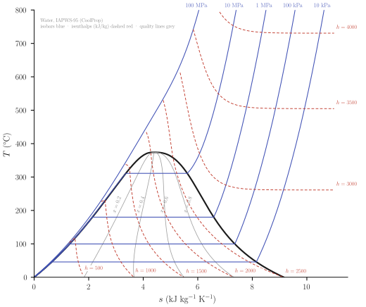
<iframe class=“webgune-interactive” src=“figures/cal-6-05.html” loading=“lazy” title=“Figure 6.5. Temperature-entropy chart for water vapor (”steam”). From Keenan, Keyes, Hill and Moore, Steam Tables, copyright © 1969, John Wiley and Sons, Inc.”>
Note that “quality” is defined as the mole fraction in the gaseous state (in the two-bhase region of the dinnen-
Each of these integrations must be carried out over a network of paths covering the entire \(T-P\) plane-often a gigantic numerical undertaking.
6-7 THE MAXIMUM PRINCIPLES FOR THE MASSIEU FUNCTIONS
In the energy representation the energy is minimum for constant entropy, and from this it follows that each Legendre transform of the energy is minimum for constant values of the transformed (intensive) variables. Similarly, in the entropy representation the entropy is maximum for constant energy, and from this it follows that each Legendre transform of the entropy is maximum for constant values of the transformed (intensive) variables.
For two of the three common Massieu functions the maximum principles can be very easily obtained, for these functions are directly related to potentials (i.e., to transforms of the energy). By equation 5.61, we have
\[ S\left[\frac{1}{T}\right]=-\frac{F}{T} \]
and, as \(F\) is minimum at constant temperature, \(S[1 / T]\) is clearly maximum. Again, by equation 5.63,
\[ S\left[\frac{1}{T}, \frac{P}{T}\right]=-\frac{G}{T} \]
and, as \(G\) is minimum at constant pressure and temperature, \(S[1 / T, P / T]\) is clearly maximum.
For the remaining common Massieu function \(S[P / T]\) we can repeat the logic of Section 6.1. We are concerned with a system in contact with a reservoir that maintains \(P / T\) constant, but permits \(1 / T\) to vary. It is readily recognized that such a reservoir is more of a mathematical fiction than a physically practical device, and the extremum principle for the function \(S[P / T]\) is correspondingly artificial. Nevertheless, the derivation of this principle along the lines of Section 6.1 is an interesting exercise that I leave to the curious reader.