STABILITY OF THERMODYNAMIC SYSTEMS
8-1 INTRINSIC STABILITY OF THERMODYNAMIC SYSTEMS
The basic extremum principle of thermodynamics implies both that \(d S=0\) and that \(d^{2} S<0\), the first of these conditions stating that the entropy is an extremum and the second stating that the extremum is, in particular, a maximum. We have not yet fully exploited the second condition, which determines the stability of predicted equilibrium states. Similarly, in classical mechanics the stable equilibrium of a rigid pendulum is at the position of minimum potential energy. A so-called “unstable equilibrium” exists at the inverted point where the potential energy is maximum.
Considerations of stability lead to some of the most interesting and significant predictions of thermodynamics. In this chapter we investigate the conditions under which a system is stable. In Chapter 9 we consider phase transitions, which are the consequences of instability.
Consider two identical subsystems, each with a fundamental equation \(S=S(U, V, N)\), separated by a totally restrictive wall. Suppose the dependence of \(S\) on \(U\) to be qualitatively as sketched in Fig. 8.1. If we were to remove an amount of energy \(\Delta U\) from the first subsystem and transfer it to the second subsystem the total entropy would change from its initial value of \(2 S(U, V, N)\) to \(S(U+\Delta U, V, N)+S(U-\Delta U, V, N)\). With the shape of the curve shown in the figure the resultant entropy would be larger than the initial entropy! If the adiabatic restraint were removed in such a system energy would flow spontaneously across the wall; one subsystem thereby would increase its energy (and its temperature) at the expense of the other. Even within one subsystem the system would find it advantageous to transfer energy from one region to another, developing internal inhomogeneities. Such a loss of homogeneity is the hallmark of a phase transition.
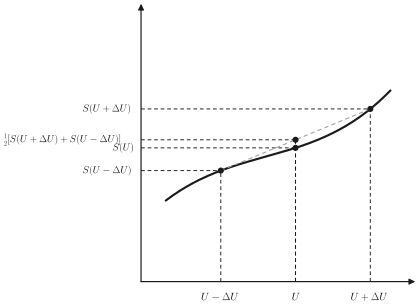
It is evident from Fig. 8.1 that the condition of stability is the concavity of the entropy. \({ }^{1}\)
\[ S(U+\Delta U, V, N)+S(U-\Delta U, V, N) \leq 2 S(U, V, N) \quad(\text { for all } \Delta) \]
For \(\Delta U \rightarrow 0\) this condition reduces to its differential form
\[ \left(\frac{\partial^{2} S}{\partial U^{2}}\right)_{V, N} \leq 0 \]
However this differential form is less restrictive than the concavity condition (8.1), which must hold for all \(\Delta U\) rather than for \(\Delta U \rightarrow 0\) only.
It is evident that the same considerations apply to a transfer of volume
\[ S(U, V+\Delta V, N)+S(U, V-\Delta V, N) \leq 2 S(U, V, N) \]
or in differential form
\[ \left(\frac{\partial^{2} S}{\partial V^{2}}\right)_{U, N} \leq 0 \]
A fundamental equation that does not satisfy the concavity conditions might be obtained from a statistical mechanical calculation or from
[^18]
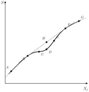
extrapolation of experimental data. The stable thermodynamic fundamental equation is then obtained from this “underlying fundamental equation” by the construction shown in Fig. 8.2. The family of tangent lines that lie everywhere above the curve (the superior tangents) are drawn; the thermodynamic fundamental equation is the envelope of these superior tangent lines.
In Fig. 8.2 the portion \(B C D E F\) of the underlying fundamental relation is unstable and is replaced by the straight line \(B H F\). It should be noted that only the portion CDE fails to satisfy the differential (or “local”) form of the stability condition (8.2), whereas the entire portion \(B C D E F\) violates the global form (8.1). The portions of the curve \(B C\) and \(E F\) are said to be “locally stable” but “globally unstable.”
A point on a straight portion ( \(B H F\) in Fig. 8.2) of the fundamental relation corresponds to a phase separation in which part of the system is in state \(B\) and part in state \(F\), as we shall see in some detail in Chapter 9.
In the three-dimensional \(S-U-V\) subspace the global condition of stability requires that the entropy surface \(S(U, V, \ldots)\) lie everywhere below its tangent planes. That is, for arbitrary \(\Delta U\) and \(\Delta V\)
\[ S(U+\Delta U, V+\Delta V, N)+S(U-\Delta U, V-\Delta V, N) \leq 2 S(U, V, N) \]
from which equations 8.2 and 8.4 again follow, as well as the additional requirement (see Problem 8.1-1) that
\[ \frac{\partial^{2} S}{\partial U^{2}} \frac{\partial^{2} S}{\partial V^{2}}-\left(\frac{\partial^{2} S}{\partial U \partial V}\right)^{2} \geqslant 0 \]
We shall soon obtain this equation by an alternative method, by applying the analogue of the simple curvature condition 8.2 to the Legendre transforms of the entropy.
To recapitulate, stability requires that the entropy surface lie everywhere below its family of tangent planes. The local conditions of stability are weaker conditions. They require not only that \(\left(\partial^{2} S / \partial U^{2}\right)_{V, N}\) and \(\left(\partial^{2} S / \partial V^{2}\right)_{U, N}\) be negative, but that \(\left[\left(\partial^{2} S / \partial U^{2}\right)\left(\partial^{2} S / \partial V^{2}\right)\right]-\) \(\left(\partial^{2} S / \partial U \partial V\right)^{2}\) must be positive. The condition \(\partial^{2} S / \partial U^{2} \leqslant 0\) ensures that the curve of intersection of the entropy surface with the plane of constant \(V\) (passing through the equilibrium point) have negative curvature. The condition \(\partial^{2} S / \partial V^{2}<0\) similarly ensures that the curve of intersection of the entropy surface with the plane of constant \(U\) have negative curvature. These two “partial curvatures” are not sufficient to ensure concavity, for the surface could be “fluted,” curving downward along the four directions \(\pm U\) and \(\pm V\), but curving upward along the four diagonal directions (between the \(U\) and \(V\) axes). It is this fluted structure that is forbidden by the third differential stability criterion (8.6).
In physical terms the local stability conditions ensure that inhomogeneities of either \(u\) or \(v\) separately do not increase the entropy, and also that a coupled inhomogeneity of \(u\) and \(v\) together does not increase the entropy.
For magnetic systems analogous relations hold, with the magnetic moment replacing the volume. \({ }^{2}\)
Before turning to the full physical implications of these stability conditions it is useful first (Section 8.2) to consider their analogues for other thermodynamic potentials. We here take note only of the most easily interpreted inequality (equation 8.3), which suggests the type of information later to be inferred from all the stability conditions. Equation 8.2 requires that
\[ \left(\frac{\partial^{2} S}{\partial U^{2}}\right)_{V, N}=-\frac{1}{T^{2}}\left(\frac{\partial T}{\partial U}\right)_{V, N}=-\frac{1}{N T^{2} c_{\nu}} \leqslant 0 \]
whence the molar heat capacity must be positive in a stable system. The remaining stability conditions will place analogous restrictions on other physically significant observables.
Finally, and in summary, in an \(r+2\) dimensional thermodynamic space \(\left(S, X_{0}, X_{1}, \ldots, X_{r}\right)\) stability requires that the entropy hyper-surface lie everywhere below its family of tangent hyper-planes.
[^19]
PROBLEMS
Problem 8.1-1
To establish the inequality 8.6 expand the left-hand side of 8.5 in a Taylor series to second order in \(\Delta U\) and \(\Delta V\). Show that this leads to the condition
\[ S_{U U}(\Delta U)^{2}+2 S_{U V} \Delta U \Delta V+S_{V V}(\Delta V)^{2} \leq 0 \]
Recalling that \(S_{U U} \equiv \partial^{2} S / \partial U^{2} \leq 0\), show that this can be written in the form
\[ \left(S_{U U} \Delta U+S_{U V} \Delta V\right)^{2}+\left(S_{U U} S_{V V}-S_{U V}^{2}\right)(\Delta V)^{2} \geqslant 0 \]
and that this condition in turn leads to equation 8.6.
Problem 8.1-2
Consider the fundamental equation of a monatomic ideal gas and show that \(S\) is a concave function of \(U\) and \(V\), and also of \(N\).
8-2 STABILITY CONDITIONS FOR THERMODYNAMIC POTENTIALS
The reformulation of the stability criteria in energy representation requires only a straightforward transcription of language. Whereas the entropy is maximum, the energy is minimum; thus the concavity of the entropy surface is replaced by convexity of the energy surface. The stable energy surface lies above its tangent planes
\[ U(S+\Delta S, V+\Delta V, N)+U(S-\Delta S, V-\Delta V, N) \geq 2 U(S, V, N) \]
The local conditions of convexity become
\[ \frac{\partial^{2} U}{\partial S^{2}}=\frac{\partial T}{\partial S} \geq 0 \quad \frac{\partial^{2} U}{\partial V^{2}}=-\frac{\partial P}{\partial V} \geq 0 \]
and for cooperative variations of \(S\) and \(V\)
\[ \frac{\partial^{2} U}{\partial S^{2}} \frac{\partial^{2} U}{\partial V^{2}}-\left(\frac{\partial^{2} U}{\partial S \partial V}\right)^{2} \geq 0 \]
This result can be extended easily to the Legendre transforms of the energy, or of the entropy. We first recall the properties of Legendre transformations (equation 5.31)
\[ P=\frac{\partial U}{\partial X} \quad \text { and } \quad X=-\frac{\partial U[P]}{\partial P} \]
whence
\[ \frac{\partial X}{\partial P}=-\frac{\partial^{2} U[P]}{\partial P^{2}}=\frac{1}{\frac{\partial^{2} U}{\partial X^{2}}} \]
Hence the sign of \(\partial^{2} U[P] / \partial P^{2}\) is the negative of the sign of \(\partial^{2} U / \partial X^{2}\). If \(U\) is a convex function of \(X\) then \(U[P]\) is a concave function of \(P\). It follows that the Helmholtz potential is a concave function of the temperature and a convex function of the volume
\[ \left(\frac{\partial^{2} F}{\partial T^{2}}\right)_{V, N} \leq 0 \quad\left(\frac{\partial^{2} F}{\partial V^{2}}\right)_{T, N} \geq 0 \]
The enthalpy is a convex function of the entropy and a concave function of the pressure
\[ \left(\frac{\partial^{2} H}{\partial S^{2}}\right)_{P, N} \geq 0 \quad\left(\frac{\partial^{2} H}{\partial P^{2}}\right)_{S, N} \leq 0 \]
The Gibbs potential is a concave function of both temperature and pressure
\[ \left(\frac{\partial^{2} G}{\partial T^{2}}\right)_{P, N} \leq 0 \quad\left(\frac{\partial^{2} G}{\partial P^{2}}\right)_{T, N} \leq 0 \]
In summary, for constant \(N\) the thermodynamic potentials (the energy and its Legendre transforms) are convex functions of their extensive variables and concave functions of their intensive variables. Similarly for constant \(N\) the Massieu functions (the entropy and its Legendre transforms) are concave functions of their extensive variables and convex functions of their intensive variables.
PROBLEMS
Problem 8.2-1
- Show that in the region \(X>0\) the function \(Y=X^{n}\) is concave for \(0<n<1\) and convex for \(n<0\) or \(n>1\).
The following four equations are asserted to be fundamental equations of physical systems. (b) \(F=A\left(\frac{N^{5} T}{V^{3}}\right)^{\frac{1}{2}}\) (c) \(G=B T^{\frac{1}{2}} P^{2} N\) (d) \(H=\frac{C S^{2} P^{\frac{1}{2}}}{N}\) (e) \(U=D\left(\frac{S^{3} V^{4}}{N^{5}}\right)^{\frac{1}{2}}\)
Which of these equations violate the criteria of stability? Assume \(A, B, C\), and \(D\) to be positive constants. Recall the “fluting condition” (equation 8.10).
Problem 8.2-2
Prove that
\[ \left(\frac{\partial^{2} F}{\partial V^{2}}\right)_{T}=\frac{\frac{\partial^{2} U}{\partial S^{2}} \frac{\partial^{2} U}{\partial V^{2}}-\left(\frac{\partial^{2} U}{\partial S \partial V}\right)^{2}}{\frac{\partial^{2} U}{\partial S^{2}}} \]
Hint: Note that \(\left(\partial^{2} F / \partial V^{2}\right)_{T}=-(\partial P / \partial V)_{T}\), and consider \(P\) formally to be a function of \(S\) and \(V\).
This identity casts an interesting perspective on the formalism. The quantity in square brackets measures the curvature of the energy along a direction intermediate between the \(S\) and \(V\) axes (recall the discussion of “fluting” after equation 8.6). The primary curvature condition on \(F\), along the \(V\) axis, is redundant with the “fluting” condition on \(U\). Only primary curvature conditions need be invoked if all potentials are considered.
Problem 8.2-3
Show that stability requires equations 8.15 and
\[ \left(\frac{\partial^{2} G}{\partial T^{2}}\right)\left(\frac{\partial^{2} G}{\partial P^{2}}\right)-\left(\frac{\partial^{2} G}{\partial T \partial P}\right)^{2} \geqslant 0 \]
(Recall Problem 8.1-1.)
8-3 PHYSICAL CONSEQUENCES OF STABILITY
We turn finally to a direct interpretation of the local stability criteria in terms of limitations on the signs of quantities such as \(c_{v}, c_{p}, \alpha\), and \(\kappa_{T}\). The first such inference was obtained in equations 8.2 or 8.7, where we found that \(c_{v} \geq 0\). Similarly, the convexity of the Helmholtz potential with respect to the volume gives
\[ \left(\frac{\partial^{2} F}{\partial V^{2}}\right)_{T}=-\left(\frac{\partial P}{\partial V}\right)_{T}=\frac{1}{V \kappa_{T}} \geq 0 \]
or
\[ \kappa_{T}>0 \]
The fact that both \(c_{v}\) and \(\kappa_{T}\) are positive (equations 8.7 and 8.17) has further implications which become evident when we recall the identities of
Problem 3.9-5
\[ c_{p}-c_{v}=\frac{T v \alpha^{2}}{\kappa_{T}} \]
and
\[ \frac{\kappa_{s}}{\kappa_{T}}=\frac{c_{v}}{c_{p}} \]
From these it follows that stability requires
\[ c_{p} \geq c_{v} \geq 0 \]
and
\[ \kappa_{T} \geq \kappa_{s} \geq 0 \]
Thus both heat capacities and both compressibilities must be positive in a stable system. Addition of heat, either at constant pressure or at constant volume, necessarily increases the temperature of a stable system-the more so at constant volume than at constant pressure. And decreasing the volume, either isothermally or isentropically, necessarily increases the pressure of a stable system-the more so isothermally than isentropically.
PROBLEMS
Problem 8.3-1
Explain on intuitive grounds why \(c_{p} \geq c_{v}\) and why \(\kappa_{T} \geq \kappa_{S}\).
Hint: Consider the energy input and the energy output during constant-pressure and constant-volume heating processes.
Problem 8.3-2
Show that the fundamental equation of a monatomic ideal gas satisfies the criteria of intrinsic stability.
Problem 8.3-3
Show that the van der Waals equation of state does not satisfy the criteria of intrinsic stability for all values of the parameters. Sketch the curves of \(P\) versus \(V\) for constant \(T\) (the isotherms of the gas) and show the region of local instability.
8-4 LE CHATELIER’S PRINCIPLE; THE QUALITATIVE EFFECT OF FLUCTUATIONS
The physical content of the stability criteria is known at Le Chatelier’s Principle. According to this principle the criterion for stability is that any inhomogeneity that somehow develops in a system should induce a process that tends to eradicate the inhomogeneity.
As an example, suppose that a container of fluid is in equilibrium and an incident photon is suddently absorbed at some point within it, locally heating the fluid slightly. Heat flows away from this heated region and, by the stability condition (that the specific heat is positive), this flow of heat tends to lower the local temperature toward the ambient value. The initial homogeneity of the system thereby is restored.
Similarly, a longitudinal vibrational wave in a fluid system induces local regions of alternately high and low density. The regions of increased density, and hence of increased pressure, tend to expand, and the regions of low density contract. The stability condition (that the compressibility is positive) ensures that these responses tend to restore the local pressure toward homogeneity.
In fact local inhomogeneities always occur in physical systems even in the absence of incident photons or of externally induced vibrations. In a gas, for instance, the individual molecules move at random, and by pure chance this motion produces regions of high density and other regions of low density.
From the perspective of statistical mechanics all systems undergo continual local fluctuations. The equilibrium state, static from the viewpoint of classical thermodynamics, is incessantly dynamic. Local inhomogeneities continually and spontaneously generate, only to be attenuated and dissipated in accordance with the Le Chatelier principle.
An informative analogy exists between a thermodynamic system and a model of a marble rolling within a “potential well.” The stable state is at the minimum of the surface. The criterion of stability is that the surface be convex.
In a slightly more sophisticated viewpoint we can conceive of the marble as being subject to Brownian motion-perhaps being buffeted by some type of random collisions. These are the mechanical analogues of the spontaneous fluctuations that occur in all real systems. The potential minimum does not necessarily coincide with the instantaneous position of the system, but rather with its “expected value”; it is this “expected value” that enters thermodynamic descriptions. The curvature of the potential well then plays a crucial and continual role, restoring the system toward the “expected state” after each Brownian impact (fluctuation). This “induced restoring force” is the content of the Le Chatelier principle.
We note in passing that in the atypical but important case in which the potential well is both shallow and asymmetric, the time-averaged position may deviate measurably from the “expected state” at the potential minimum. In such a case classical thermodynamics makes spurious predictions which deviate from observational data, for thermodynamic measurements yield average values (recall Chapter 1). Such a pathological case arises at higher-order phase transitions-the correct theory of which was developed in the 1970s. We shall explore that area in Chapter 11.
8-5 THE LE CHATELIER-BRAUN PRINCIPLE
Returning to the physical interpretation of the stability criteria, a more subtle insight than that given by the Le Chatelier principle is formulated in the Le Chatelier-Braun principle.
Consider a system that is taken out of equilibrium by some action or fluctuation. According to the Le Chatelier principle the perturbation directly induces a process that attenuates the perturbation. But various other secondary processes are also induced, indirectly. The content of the Le Chatelier-Braun principle is that these indirectly induced processes also act to attenuate the initial perturbation.
A simple example may clarify the principle. Consider a subsystem contained within a cylinder with diathermal walls and a loosely fitting piston, all immersed within a “bath” (a thermal and pressure reservoir). The piston is moved outward slightly, either by an external agent or by a fluctuation. The primary effect is that the internal pressure is decreased-the pressure difference across the piston then acts to push it inward; this is the Le Chatelier principle. A second effect is that the initial expansion \(d V\) alters the temperature of the subsystem; \(d T=\) \((\partial T / \partial V)_{S} d V=-\left(T \alpha / N c_{v} \kappa_{T}\right) d V\). This change of temperature may have either sign, depending on the sign of \(\alpha\). Consequently there is a flow of heat through the cylinder walls, inward if \(\alpha\) is positive and outward if \(\alpha\) is negative (sign \(d Q=\operatorname{sign} \alpha\) ). This flow of heat, in turn, tends to change the pressure of the system: \(d P=(1 / T)(\partial P / \partial S)_{V} d Q=\left(\alpha / N T^{2} c_{v} \kappa_{T}\right) d Q\). The pressure is increased for either sign of \(\alpha\). Thus a secondary induced process (heat flow) also acts to diminish the initial perturbation. This is the Le Chatelier-Braun principle.
To demonstrate both the Le Chatelier and the Le Chatelier-Braun principles formally, let a spontaneous fluctuation \(d X_{1}^{f}\) occur in a composite system. This fluctuation is accompanied by a change in the intensive parameter \(P_{1}\) of the subsystem
\[ d P_{1}^{f}=\frac{\partial P_{1}}{\partial X_{1}} d X_{1}^{f} \]
The fluctuation \(d X_{1}^{f}\) also alters the intensive parameter \(P_{2}\)
\[ d P_{2}^{f}=\frac{\partial P_{2}}{\partial X_{1}} d X_{1}^{f} \]
Now we can inquire as to the changes in \(X_{1}\) and \(X_{2}\) which are driven by these two deviations \(d P_{1}^{f}\) and \(d P_{2}^{f}\). We designate the driven change in \(d X_{1}\) by \(d X_{j}^{r}\), the superscript indicating “response.” The signs of \(d X_{1}^{r}\) and \(d X_{2}^{r}\) are determined by the minimization of the total energy (at constant total entropy)
\[ \begin{aligned} d\left(U+U^{\mathrm{res}}\right) & =\left(P_{1}-P_{1}^{\mathrm{res}}\right) d X_{1}^{r}+\left(P_{2}-P_{2}^{\mathrm{res}}\right) d X_{2}^{r} \leq 0 \\ & =d P_{1}^{f} d X_{1}^{r}+d P_{2}^{f} d X_{2}^{r} \leq 0 \end{aligned} \]
Hence, since \(d X_{1}^{r}\) and \(d X_{2}^{r}\) are independent
\[ d P_{1}^{f} d X_{1}^{r} \leq 0 \]
and
\[ d P_{2}^{f} d X_{2}^{r} \leq 0 \]
From the first of these and equation 8.22
\[ \frac{d P_{1}}{d X_{1}} d X_{1}^{f} d X_{1}^{r} \leq 0 \]
and similarly
\[ \frac{d P_{2}}{d X_{1}} d X_{1}^{f} d X_{2}^{f} \leq 0 \]
We examine these two results in turn. The first, equation 8.28, is the formal statement of the Le Chatelier principle. For multiplying by \(d P_{1} / d X_{1}\), which is positive by virtue of the convexity criterion of stability,
\[ \frac{d P_{1}}{d X_{1}} d X_{1}^{f} \cdot \frac{d P_{1}}{d X_{1}} d X_{1}^{r} \leq 0 \]
or
\[ d P_{1}^{f} d P_{1}^{r(1)} \leq 0 \]
That is, the response \(d X_{1}^{r}\) produces a change \(d P_{1}^{r(1)}\) in the intensive parameter \(P_{1}\) that is opposite in sign to the change \(d P_{1}^{f}\) induced by the initial fluctuation.
The second inequality, (8.29), can be rewritten by the Maxwell relation
\[ \frac{\partial P_{2}}{\partial X_{1}}=\frac{\partial P_{1}}{\partial X_{2}} \]
in the form
\[ d X_{1}^{f} \cdot\left(\frac{\partial P_{1}}{\partial X_{2}} d X_{2}^{r}\right) \leq 0 \]
Then, multiplying by the positive quantity \(d P_{1} / d X_{1}\)
\[ \left(\frac{\partial P_{1}}{\partial X_{1}} d X_{1}^{f}\right)\left(\frac{d P_{1}}{d X_{2}} d X_{2}^{r}\right) \leq 0 \]
or
\[ \left(d P_{1}^{f}\right)\left(d P_{1}^{r(2)}\right) \leq 0 \]
That is, the response \(d X_{2}^{r}\) produces a change \(d P_{1}^{r(2)}\) in the intensive parameter \(P_{1}\) which is opposite in sign to the change in \(P_{1}\) directly induced by the initial fluctuation. This is the Le Chatelier-Braun principle.
Finally, it is of some interest to note that equation 8.33 is subject to another closely correlated interpretation. Multiplying by the positive quantity \(d P_{2} / d X_{2}\)
\[ \left(\frac{\partial P_{2}}{\partial X_{1}} d X_{1}^{f}\right)\left(\frac{\partial P_{2}}{\partial X_{2}} d X_{2}^{r}\right) \leq 0 \]
or
\[ \left(d P_{2}^{f}\right)\left(d P_{2}^{r(2)}\right) \leq 0 \]
That is, the response in \(X_{2}\) produces a change in \(P_{2}\) opposite in sign to the change induced by the initial fluctuation in \(X_{1}\).
PROBLEMS
Problem 8.5-1
A system is in equilibrium with its environment at a common temperature and a common pressure. The entropy of the system is increased slightly (by a fluctuation in which heat flows into the system, or by the purposeful injection of heat into the system). Explain the implications of both the Le Chatelier and the Le Chatelier-Braun principles to the ensuing processes, proving your assertions in detail.