SOME FORMAL RELATIONSHIPS, AND SAMPLE SYSTEMS
3-1 THE EULER EQUATION
Having seen how the fundamental postulates lead to a solution of the equilibrium problem, we now pause to examine in somewhat greater detail the mathematical properties of fundamental equations.
The homogeneous first-order property of the fundamental relation permits that equation to be written in a particularly convenient form, called the Euler form. From the definition of the homogeneous first-order property we have, for any \(\lambda\)
\[ U\left(\lambda S, \lambda X_{1}, \ldots, \lambda X_{t}\right)=\lambda U\left(S, X_{1}, \ldots, X_{t}\right) \]
Differentiating with respect to \(\lambda\)
\[ \begin{aligned} & \frac{\partial U\left(\ldots, \lambda X_{k}, \ldots\right)}{\partial(\lambda S)} \frac{\partial(\lambda S)}{\partial \lambda}+\frac{\partial U\left(\ldots, \lambda X_{k}, \ldots\right)}{\partial\left(\lambda X_{j}\right)} \frac{\partial\left(\lambda X_{j}\right)}{\partial \lambda} \\ & \quad+\cdots=U\left(S, X_{1}, \ldots, X_{t}\right) \end{aligned} \]
or
\[ \begin{aligned} & \frac{\partial U\left(\ldots, \lambda X_{k}, \ldots\right)}{\partial(\lambda S)} S+\sum_{j=1}^{t} \frac{\partial U\left(\ldots, \lambda X_{k}, \ldots\right)}{\partial\left(\lambda X_{j}\right)} X_{j} \\ & \quad=U\left(S, X_{1}, \ldots, X_{t}\right) \end{aligned} \]
This equation is true for any \(\lambda\) and in particular for \(\lambda=1\), in which case it takes the form
\[ \begin{gathered} \frac{\partial U}{\partial S} S+\sum_{j=1}^{t} \frac{\partial U}{\partial X_{j}} X_{j}+\cdots=U \\ U=T S+\sum_{j=1}^{t} P_{j} X_{j} \end{gathered} \]
For a simple system in particular we have
\[ U=T S-P V+\mu_{1} N_{1}+\cdots+\mu_{r} N_{r} \]
The relation 3.5 or 3.6 is the particularization to thermodynamics of the Euler theorem on homogeneous first-order forms. The foregoing development merely reproduces the standard mathematical derivation. We refer to equation 3.5 or 3.6 as the Euler relation.
In the entropy representation the Euler relation takes the form
\[ S=\sum_{j=0}^{t} F_{j} X_{j} \]
or
\[ S=\left(\frac{1}{T}\right) U+\left(\frac{P}{T}\right) V-\sum_{k=1}^{r}\left(\frac{\mu_{k}}{T}\right) N_{k} \]
PROBLEMS
Problem 3.1-1
Write each of the five physically acceptable fundamental equations of Problem 1.10-1 in the Euler form.
3-2 THE GIBBS-DUHEM RELATION
In Chapter 2 we arrived at equilibrium criteria involving the temperature, pressure, and chemical potentials. Each of the intensive parameters entered the theory in a similar way, and the formalism is, in fact, symmetric in the several intensive parameters. Despite this symmetry, however, the reader is apt to feel an intuitive response to the concepts of temperature and pressure, which is lacking, at least to some degree, in the case of the chemical potential. It is of interest, then, to note that the intensive parameters are not all independent. There is a relation among the intensive parameters, and for a single-component system \(\mu\) is a function of \(T\) and \(P\).
The existence of a relationship among the various intensive parameters is a consequence of the homogeneous first-order property of the fundamental relation. For a single-component system this property permits the fundamental relation to be written in the form \(u=u(s, v)\), as in equation 2.19; each of the three intensive parameters is then also a function of \(s\) and \(v\). Elimination of \(s\) and \(v\) from among the three equations of state yields a relation among \(T, P\), and \(\mu\).
The argument can easily be extended to the more general case, and it again consists of a straightforward counting of variables. Suppose we have a fundamental equation in \((t+1)\) extensive variables
\[ U=U\left(S, X_{1}, X_{2}, \ldots, X_{t}\right) \]
yielding, in turn, \(t+1\) equations of state
\[ P_{k}=P_{k}\left(S, X_{1}, X_{2}, \ldots, X_{t}\right) \]
If we choose the parameter \(\lambda\) of equation 2.14 as \(\lambda=1 / X_{t}\), we then have
\[ P_{k}=P_{k}\left(S / X_{t}, X_{1} / X_{t}, \ldots, X_{t-1} / X_{t}, 1\right) \]
Thus each of the \((t+1)\) intensive parameters is a function of just \(t\) variables. Elimination of these \(t\) variables among the \((t+1)\) equations yields the desired relation among the intensive parameters.
To find the explicit functional relationship that exists among the set of intensive parameters would require knowledge of the explicit fundamental equation of the system. That is, the analytic form of the relationship varies from system to system. Given the fundamental relation, the procedure is evident and follows the sequence of steps indicated by equations 3.9 through 3.11.
A differential form of the relation among the intensive parameters can be obtained directly from the Euler relation and is known as the Gibbs-Duhem relation. Taking the infinitesimal variation of equation 3.5, we find
\[ d U=T d S+S d T+\sum_{j=1}^{t} P_{j} d X_{j}+\sum_{j=1}^{t} X_{j} d P_{j} \]
But, in accordance with equation 2.6, we certainly know that
\[ d U=T d S+\sum_{j=1}^{t} P_{j} d X_{j} \]
whence, by subtraction we find the Gibbs-Duhem relation
\[ S d T+\sum_{j=1}^{t} X_{j} d P_{j}=0 \]
For a single-component simple system, in particular, we have
\[ S d T-V d P+N d \mu=0 \]
or
\[ d \mu=-s d T+v d P \]
The variation in chemical potential is not independent of the variations in temperature and pressure, but the variation of any one can be computed in terms of the variations of the other two.
The Gibbs-Duhem relation presents the relationship among the intensive parameters in differential form. Integration of this equation yields the relation in explicit form, and this is a procedure alternative to that presented in equations 3.9 through 3.11. In order to integrate the Gibbs-Duhem relation, one must know the equations of state that enable one to write the \(X_{j}\) ’s in terms of the \(P_{j}\) ’s, or vice versa.
The number of intensive parameters capable of independent variation is called the number of thermodynamic degrees of freedom of a given system. A simple system of \(r\) components has \(r+1\) thermodynamic degrees of
In the entropy representation the Gibbs-Duhem relation again states freedom. that the sum of products of the extensive parameters and the differentials of the corresponding intensive parameters vanishes.
\[ \sum_{j=0}^{t} X_{j} d F_{j}=0 \]
or
\[ U d\left(\frac{1}{T}\right)+V d\left(\frac{P}{T}\right)-\sum_{k=1}^{r} N_{k} d\left(\frac{\mu_{k}}{T}\right)=0 \]
PROBLEMS
Problem 3.2-1
Find the relation among \(T, P\), and \(\mu\) for the system with the fundamental equation
\[ U=\left(\frac{v_{0}^{2} \theta}{R^{3}}\right) \frac{S^{4}}{N V^{2}} \]
3-3 SUMMARY OF FORMAL STRUCTURE
Let us now summarize the structure of the thermodynamic formalism in the energy representation. For the sake of clarity, and in order to be explicit, we consider a single-component simple system. The fundamental equation
\[ U=U(S, V, N) \]
contains all thermodynamic information about a system. With the definitions \(T=\partial U / \partial S\), and so forth, the fundamental equation implies three equations of state
\[ \begin{aligned} & T=T(S, V, N)=T(s, v) \\ & P=P(S, V, N)=P(s, v) \\ & \mu=\mu(S, V, N)=\mu(s, v) \end{aligned} \]
If all three equations of state are known, they may be substituted into the Euler relation, thereby recovering the fundamental equation. Thus the totality of all three equations of state is equivalent to the fundamental equation and contains all thermodynamic information about a system. Any single equation of state contains less thermodynamic information than the fundamental equation.
If two equations of state are known, the Gibbs-Duhem relation can be integrated to obtain the third. The equation of state so obtained will contain an undetermined integration constant. Thus two equations of state are sufficient to determine the fundamental equation, except for an undetermined constant.
A logically equivalent but more direct and generally more convenient method of obtaining the fundamental equation when two equations of state are given is by direct integration of the molar relation
\[ d u=T d s-P d v \]
Clearly, knowledge of \(T=T(s, v)\) and \(P=P(s, v)\) yields a differential equation in the three variables \(u, s\), and \(v\), and integration gives
\[ u=u(s, v) \]
which is a fundamental equation. Again, of course, we have an undetermined constant of integration.
It is always possible to express the internal energy as a function of parameters other than \(S, V\), and \(N\). Thus we could eliminate \(S\) from \(U=U(S, V, N)\) and \(T=T(S, V, N)\) to obtain an equation of the form \(U=U(T, V, N)\). However, I stress that such an equation is not a fundamental relation and does not contain all possible thermodynamic informa-
tion about the system. In fact, recalling the definition of \(T\) as \(\partial U / \partial S\), we see that \(U=U(T, V, N)\) actually is a partial differential equation. Even if this equation were integrable, it would yield a fundamental equation with undetermined functions. Thus knowledge of the relation \(U=U(S, V, N)\) allows one to compute the relation \(U=U(T, V, N)\), but knowledge of \(U=U(T, V, N)\) does not permit one inversely to compute \(U=\) \(U(S, V, N)\). Associated with every equation there is both a truth value and an informational content. Each of the equations \(U=U(S, V, N)\) and \(U=U(T, V, N)\) may be true, but only the former has the optimum informational content.
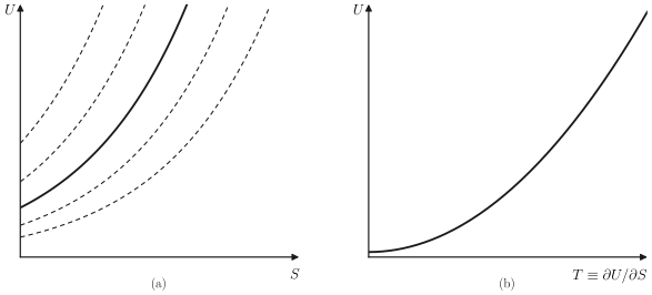
These statements are graphically evident if we focus, for instance, on the dependence of \(U\) on \(S\) at constant \(V\) and \(N\). Let that dependence be as shown in the solid curve in Fig. 3.1(a). This curve uniquely determines the dependence of \(U\) on \(T\), shown in Fig. 3.1(b); for each point on the \(U(S)\) curve there is a definite \(U\) and a definite slope \(T=\partial U / \partial S\), determining a point on the \(U(T)\) curve. Suppose, however, that we are given the \(U(T)\) curve (an equation of state) and we seek to recover the fundamental \(U(S)\) curve. Each of the dotted curves in Fig. 3.1(a) is equally compatible with the given \(U(T)\) curve, for all have the same slope \(T\) at a given \(U\). The curves differ by an arbitrary displacement, corresponding to the arbitrary “constant of integration” in the solution of the differential equation \(U=U(\partial U / \partial S)\). Thus, Fig. 3.1(a) implies Fig. 3.1(b), but the reverse is not true. Equivalently stated, only \(U=U(S)\) is a fundamental relation. The formal structure is illustrated by consideration of several specific and explicit systems in the following Sections of this book.
Example
A particular system obeys the equations
\[ U=\frac{1}{2} P V \]
and
\[ T^{2}=\frac{A U^{3 / 2}}{V N^{1 / 2}} \]
where \(A\) is a positive constant. Find the fundamental equation. Solution Writing the two equations in the form of equations of state in the entropy representation (which is suggested by the appearance of \(U, V\), and \(N\) as independent parameters)
\[ \begin{aligned} & \frac{1}{T}=A^{-1 / 2} u^{-3 / 4} v^{1 / 2} \\ & \frac{P}{T}=2 A^{-1 / 2} u^{1 / 4} v^{-1 / 2} \end{aligned} \]
Then the differential form of the molar fundamental equation (the analogue of equation 3.23) is so that
\[ \begin{aligned} d s & =\frac{1}{T} d u+\frac{P}{T} d v \\ & =A^{-1 / 2}\left(u^{-3 / 4} v^{1 / 2} d u+2 u^{1 / 4} v^{-1 / 2} d v\right) \\ & =4 A^{-1 / 2} d\left(u^{1 / 4} v^{1 / 2}\right) \end{aligned} \]
and
\[ s=4 A^{-1 / 2} u^{1 / 4} v^{1 / 2}+s_{0} \]
\[ S=4 A^{-1 / 2} U^{1 / 4} V^{1 / 2} N^{1 / 4}+N s_{0} \]
The reader should compare this method with the alternative technique of first integrating the Gibbs-Duhem relation to obtain \(\mu(u, v)\), and then inserting the three equations of state into the Euler equation.
Particular note should be taken of the manner in which \(d s\) is integrated to obtain \(s\). The equation for \(d s\) in terms of \(d u\) and \(d v\) is a partial differential equation-it certainly cannot be integrated term by term, nor by any of the familiar methods for ordinary differential equations in one independent variable. We have integrated the equation by “inspection”; simply “recognizing” that \(u^{-3 / 4} v^{1 / 2} d u+2 u^{1 / 4} v^{-1 / 2} d v\) is the differential of \(u^{1 / 4} v^{1 / 2}\).
PROBLEMS
Problem 3.3-1
A particular system obeys the two equations of state
\[ T=\frac{3 A s^{2}}{v}, \quad \text { the thermal equation of state } \]
and
\[ P=\frac{A s^{3}}{v^{2}}, \quad \text { the mechanical equation of state } \]
where \(A\) is constant.
Find \(\mu\) as a function of \(s\) and \(v\), and then find the fundamental equation.
Find the fundamental equation of this system by direct integration of the molar form of the equation.
Problem 3.3-2
It is found that a particular system obeys the relations
\[ U=P V \]
and
\[ P=B T^{2} \]
where \(B\) is constant. Find the fundamental equation of this system.
Problem 3.3-3
A system obeys the equations
\[ P=-\frac{N U}{N V-2 A V U} \]
and
\[ T=2 C \frac{U^{1 / 2} V^{1 / 2}}{N-2 A U} e^{A U / N} \]
Find the fundamental equation. Hint: To integrate, let
\[ s=D u^{n} v^{m} e^{-A u} \]
where \(D, n\), and \(m\) are constants to be determined.
Problem 3.3-4
A system obeys the two equations \(u=\frac{3}{2} P v\) and \(u^{1 / 2}=B T v^{1 / 3}\). Find the fundamental equation of this system.
3-4 THE SIMPLE IDEAL GAS AND MULTICOMPONENT SIMPLE IDEAL GASES
A “simple ideal gas” is characterized by the two equations
\[ P V=N R T \]
and
\[ U=c N R T \]
where \(c\) is a constant and \(R\) is the “universal gas constant” ( \(R=N_{A} k_{B}=\) 8.3144 J/mole K).
Gases composed of noninteracting monatomic atoms (such as He, Ar, Ne ) are observed to satisfy equations 3.25 and 3.26 at temperatures such that \(k_{B} T\) is small compared to electronic excitation energies (i.e., \(T \lesssim 10^{4}\) K), and at low or moderate pressures. All such “monatomic ideal gases” have a value of \(c=\frac{3}{2}\).
Under somewhat more restrictive conditions of temperature and pressure other real gases may conform to the simple ideal gas equations 3.25 and 3.26, but with other values of the constant \(c\). For diatomic molecules (such as \(\mathrm{O}_{2}\) or NO) there tends to be a considerable region of temperature for which \(c \simeq \frac{5}{2}\) and another region of higher temperature for which \(c \simeq \frac{7}{2}\) (with the boundary between these regions generally occurring at temperatures on the order of \(10^{3} \mathrm{~K}\) ).
Equations 3.25 and 3.26 permit us to determine the fundamental equation. The explicit appearance of the energy \(U\) in one equation of state (equation 3.26) suggests the entropy representation. Rewriting the equations in the correspondingly appropriate form
\[ \frac{1}{T}=c R\left(\frac{N}{U}\right)=\frac{c R}{u} \]
and
\[ \frac{P}{T}=R\left(\frac{N}{V}\right)=\frac{R}{v} \]
From these two entropic equations of state we find the third equation of state
\[ \frac{\mu}{T}=\text { function of } u, v \]
by integration of the Gibbs-Duhem relation
\[ d\left(\frac{\mu}{T}\right)=u d\left(\frac{1}{T}\right)+v d\left(\frac{P}{T}\right) \]
Finally, the three equations of state will be substituted into the Euler equation
\[ S=\left(\frac{1}{T}\right) U+\left(\frac{P}{T}\right) V-\left(\frac{\mu}{T}\right) N \]
Proceeding in this way the Gibbs-Duhem relation (3.30) becomes
\[ d\left(\frac{\mu}{T}\right)=u \times\left(-\frac{c R}{u^{2}}\right) d u+v \times\left(-\frac{R}{v^{2}}\right) d v=-c R \frac{d u}{u}-R \frac{d u}{v} \]
and integrating
\[ \frac{\mu}{T}-\left(\frac{\mu}{T}\right)_{0}=-c R \ln \frac{u}{u_{0}}-R \ln \frac{v}{v_{0}} \]
Here \(u_{0}\) and \(v_{0}\) are the parameters of a fixed reference state, and \((\mu / T)_{0}\) arises as an undetermined constant of integration. Then, from the Euler relation (3.31)
\[ S=N s_{0}+N R \ln \left[\left(\frac{U}{U_{0}}\right)^{c}\left(\frac{V}{V_{0}}\right)\left(\frac{N}{N_{0}}\right)^{-(c+1)}\right] \]
where
\[ s_{0}=\left(c+\frac{1}{3}\right) R-\left(\frac{\mu}{T}\right)_{0} \]
Equation 3.34 is the desired fundamental equation; if the integration constant \(s_{0}\) were known equation 3.34 would contain all possible thermodynamic information about a simple ideal gas.
This procedure is neither the sole method, nor even the preferred method. Alternatively, and more directly, we could integrate the molar equation
\[ d s=\left(\frac{1}{T}\right) d u+\left(\frac{P}{T}\right) d v \]
which, in the present case, becomes
\[ d s=c\left(\frac{R}{u}\right) d u+\left(\frac{R}{v}\right) d v \]
giving, on integration,
\[ s=s_{0}+c R \ln \left(\frac{u}{u_{0}}\right)+R \ln \left(\frac{v}{v_{0}}\right) \]
This equation is equivalent to equation 3.34. It should, perhaps, be noted that equation 3.37 is integrable term by term, despite our injunction (in Example 3) that such an approach generally is not possible. The segregation of the independent variables \(u\) and \(v\) in separate terms in equation 3.37 is a fortunate but unusual simplification which permits term by term integration in this special case.
A mixture of two or more simple ideal gases-a “multicomponent simple ideal gas”-is characterized by a fundamental equation which is most simply written in parametric form, with the temperature \(T\) playing the role of the parametric variable.
\[ \begin{aligned} & S=\sum_{j} N_{j} s_{j 0}+\left(\sum_{j} N_{j} c_{j}\right) R \ln \frac{T}{T_{0}}+\sum_{j} N_{j} R \ln \left(\frac{V}{N_{j} v_{0}}\right) \\ & U=\left(\sum_{j} N_{j} c_{j}\right) R T \end{aligned} \]
Elimination of \(T\) between these equations gives a single equation of the standard form \(S=S\left(U, V, N_{1}, N_{2}, \ldots\right)\).
Comparison of the individual terms of equations 3.39 with the expression for the entropy of a single-component ideal gas leads to the following interpretation (often referred to as Gibbs’s Theorem). The entropy of a mixture of ideal gases is the sum of the entropies that each gas would have if it alone were to occupy the volume \(V\) at temperature \(T\). The theorem is, in fact, true for all ideal gases (Chapter 13).
It is also of interest to note that the first of equations 3.39 can be written in the form
\[ S=\sum_{j} N_{j} s_{j 0}+\left(\sum_{j} N_{j} c_{j}\right) R \ln \frac{T}{T_{0}}+N R \ln \frac{V}{N v_{0}}-R \sum_{j} N_{j} \ln \frac{N_{j}}{N} \]
and the last term is known as the “entropy of mixing.” It represents the difference in entropies between that of a mixture of gases and that of a collection of separate gases each at the same temperature and the same density as the original mixture \(N_{j} / V_{j}=N / V\), (and hence at the same pressure as the original mixture); see Problem 3.4-15. The close similarity, and the important distinction, between Gibbs’s theorem and the interpretation of the entropy of mixing of ideal gases should be noted carefully by the reader. An application of the entropy of mixing to the problem of isotope separation will be given in Section 4.4 (Example 4).
Gibbs’s theorem is demonstrated very neatly by a simple “thought experiment.” A cylinder (Fig. 3.2) of total volume \(2 V_{0}\) is divided into four chambers (designated as \(\alpha, \beta, \gamma, \delta\) ) by a fixed wall in the center and by two sliding walls. The two sliding walls are coupled together so that their distance apart is always one half the length of the cylinder ( \(V_{\alpha}=V_{\gamma}\) and \(\left.V_{\beta}=V_{\delta}\right)\). Initially, the two sliding walls are coincident with the left end and the central fixed partition, respectively, so that \(V_{\alpha}=V_{\gamma}=0\). The chamber \(\beta\), of volume \(V_{0}\), is filled with a mixture of \(N_{0}\) moles of a simple ideal gas \(A\) and \(N_{0}\) moles of a simple ideal gas \(B\). Chamber \(\delta\) is initially evacuated. The entire system is maintained at temperature \(T\).
The left-hand sliding wall is permeable to component \(A\), but not to component \(B\). The fixed partition is permeable to component \(B\), but not to component \(A\). The right-hand sliding wall is impermeable to either component.
The coupled sliding walls are then pushed quasi-statically to the right until \(V_{\beta}=V_{\delta}=0\) and \(V_{\alpha}=V_{\gamma}=V_{0}\). Chamber \(\alpha\) then contains pure \(A\) and chamber \(\gamma\) contains pure \(B\). The initial mixture, of volume \(V_{0}\), thereby is separated into two pure components, each of volume \(V_{0}\). According to Gibbs’s theorem the final entropy should be equal to the initial entropy, and we shall now see directly that this is, in fact, true.
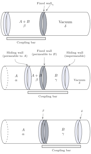
We first note that the second of equations 3.39, stating that the energy is a function of only \(T\) and the mole number, ensures that the final energy is equal to the initial energy of the system. Thus \(-T \Delta S\) is equal to the work done in moving the coupled walls.
The condition of equilibrium with respect to transfer of component \(A\) across the left-hand wall is \(\mu_{A, \alpha}=\mu_{A, \beta}\). It is left to Problem 3.4-14 to show that the conditions \(\mu_{A, \alpha}=\mu_{A, \beta}\) and \(\mu_{B, \beta}=\mu_{B, \gamma}\) imply that
\[ P_{\alpha}=P_{\gamma} \text { and } P_{\beta}=2 P_{\alpha} \]
That is, the total force on the coupled moveable walls \(\left(P_{\alpha}-P_{\beta}+P_{\gamma}\right)\) vanishes. Thus no work is done in moving the walls, and consequently no entropy change accompanies the process. The entropy of the original mixture of \(A\) and \(B\), in a common volume \(V_{0}\), is precisely equal to the entropy of pure \(A\) and pure \(B\), each in a separate volume \(V_{0}\). This is Gibbs’s theorem.
Finally, we note that the simple ideal gas considered in this section is a special case of the general ideal gas, which encompasses a very wide class of real gases at low or moderate pressures. The general ideal gas is again characterized by the mechanical equation of state \(P V=N R T\) (equation 3.25), and by an energy that again is a function of the temperature only-but not simply a linear function. The general ideal gas will be discussed in detail in Chapter 13, and statistical mechanical derivations of the fundamental equations will emerge in Chapter 16.
PROBLEMS
Note that Problems 3.4-1, 3.4-2, 3.4-3, and 3.4-8 refer to “quasi-static processes”; such processes are to be interpreted not as real processes but merely as loci of equilibrium states. Thus we can apply thermodynamics to such quasi-static “processes”; the work done in a quasi-static change of volume (from \(V_{1}\) to \(V_{2}\) ) is \(W=-\int P d V\) and the heat transfer is \(Q=\int T d S\). The relationship of real processes to these idealized “quasi-static processes” will be discussed in Chapter 4.
Problem 3.4-1
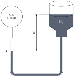
A “constant volume ideal gas thermometer” is constructed as shown (schematically) in Fig. 3.3. The bulb containing the gas is constructed of a material with a negligibly small coefficient of thermal expansion. The point \(A\) is a reference point marked on the stem of the bulb. The bulb is connected by a flexible tube to a reservoir of liquid mercury, open to the atmosphere.. The mercury reservoir is raised or lowered until the mercury miniscus coincides with the reference point \(A\). The height \(h\) of the mercury column is then read.
Show that the pressure of the gas is the sum of the external (atmospheric) pressure plus the height \(h\) of the mercury column multiplied by the weight per unit volume of mercury (as measured at the temperature of interest).
Using the equation of state of the ideal gas, explain how the temperature of the gas is then evaluated.
- Describe a “constant pressure ideal gas thermometer” (in which a changing volume is directly measured at constant pressure).
Problem 3.4-2
Show that the relation between the volume and the pressure of a monatomic ideal gas undergoing a quasi-static adiabatic compression \((d Q=T d S=0\). \(S=\) constant \()\) is
\[ P v^{5 / 3}=\left(P_{0} v_{0}^{5 / 3} e^{-2 s_{0} / 3 R}\right) e^{2 s / 3 R}=\text { constant } \]
Sketch a family of such “adiabats” in a graph of \(P\) versus \(V\). Find the corresponding relation for a simple ideal gas.
Problem 3.4-3
Two moles of a monatomic ideal gas are at a temperature of 0°C and a volume of 45 liters. The gas is expanded adiabatically ( \(d Q=0\) ) and quasi-statically until its temperature falls to -50°C. What are its initial and final pressures and its final volume?
Answer:
\[ P_{t}=0.1 \mathrm{MPa}, V_{f}=61 \times 10^{-3} \mathrm{~m}^{3} \]
Problem 3.4-4
By carrying out the integral \(\int P d V\), compute the work done by the gas in Problem 3.4-3. Also compute the initial and final energies, and corroborate that the difference in these energies is the work done.
Problem 3.4-5
In a particular engine a gas is compressed in the initial stroke of the piston. Measurements of the instantaneous temperature, carried out during the compression, reveal that the temperature increases according to
\[ T=\left(\frac{V}{V_{0}}\right)^{\eta} T_{0} \]
where \(T_{0}\) and \(V_{0}\) are the initial temperature and volume, and \(\eta\) is a constant. The gas is compressed to the volume \(V_{1}\) (where \(V_{1}<V_{0}\) ). Assume the gas to be monatomic ideal, and assume the process to be quasi-static.
Calculate the work \(W\) done on the gas.
Calculate the change in energy \(\Delta U\) of the gas.
Calculate the heat transfer \(Q\) to the gas (through the cylinder walls) by using the results of ( \(a\) ) and ( \(b\) ).
Calculate the heat transfer directly by integrating \(d Q=T d S\). \(e\) ) From the result of ( \(c\) ) or ( \(d\) ), for what value of \(\eta\) is \(Q=0\) ? Show that for this value of \(\eta\) the locus traversed coincides with an adiabat (as calculated in Problem 3.4-2).
Problem 3.4-6
Find the three equations of state of the “simple ideal gas” (equation 3.34). Show that these equations of state satisfy the Euler relation.
Problem 3.4-7
Find the four equations of state of a two-component mixture of simple ideal gases (equations 3.39). Show that these equations of state satisfy the Euler relation.
Problem 3.4-8
If a monatomic ideal gas is permitted to expand into an evacuated region, thereby increasing its volume from \(V\) to \(\lambda V\), and if the walls are rigid and adiabatic, what is the ratio of the initial and final pressures? What is the ratio of the initial and final temperatures? What is the difference of the initial and final entropies?
Problem 3.4-9
A tank has a volume of \(0.1 \mathrm{~m}^{3}\) and is filled with He gas at a pressure of \(5 \times 10^{6} \mathrm{~Pa}\). A second tank has a volume of \(0.15 \mathrm{~m}^{3}\) and is filled with He gas at a pressure of \(6 \times 10^{6} \mathrm{~Pa}\). A valve connecting the two tanks is opened. Assuming He to be a monatomic ideal gas and the walls of the tanks to be adiabatic and rigid, find the final pressure of the system.
Hint: Note that the internal energy is constant.
Answer:
\[ P_{f}=5.6 \times 10^{6} \mathrm{~Pa} \]
3.4-10.
If the temperatures within the two tanks of Problem 3.4-9, before opening the valve, had been \(T=300 \mathrm{~K}\) and 350 K , respectively, what would the final temperature be?
If the first tank had contained He at an initial temperature of 300 K , and the second had contained a diatomic ideal gas with \(c=5 / 2\) and an initial temperature of 350 K , what would the final temperature be?
Answer:
\(T_{f}=330 \mathrm{~K}\)
\(T_{f}=337 \mathrm{~K}\)
Problem 3.4-11
Show that the pressure of a multicomponent simple ideal gas can be written as the sum of “partial pressures” \(P_{j}\), where \(P_{j} \equiv N_{j} R T / V\). These “partial pressures” are purely formal quantities not subject to experimental observation. (From the mechanistic viewpoint of kinetic theory the partial pressure \(P_{t}\) is the contribution to the total pressure that results from bombardment of the wall by molecules of species \(i\)-a distinction that can be made only when the molecules are noninteracting, as in an ideal gas.)
Problem 3.4-12
Show that \(\mu_{j}\), the electrochemical potential of the \(j\) th component in a multicomponent simple ideal gas, satisfies
\[ \mu_{j}=R T \ln \left(\frac{N_{j} v_{0}}{V}\right)+(\text { function of } T) \]
and find the explicit form of the “function of \(T\).” Show that \(\mu\), can be expressed in terms of the “partial pressure” (Problem 3.4-11) and the temperature.
Problem 3.4-13
An impermeable, diathermal, and rigid partition divides a container into two subvolumes, each of volume \(V\). The subvolumes contain, respectively, one
mole of \(\mathrm{H}_{2}\) and three moles of Ne. The system is maintained at constant temperature \(T\). The partition is suddenly made permeable to \(\mathrm{H}_{2}\), but not to Ne, and equilibrium is allowed to reestablish. Find the mole numbers and the pressures.
Problem 3.4-14
Use the results of Problems 3.4-11 and 3.4-12 to establish the results \(P_{\alpha}=P_{\gamma}\) and \(P_{\beta}=2 P_{\alpha}\) in the demonstration of Gibbs’s theorem at the end of this section.
Problem 3.4-15
An impermeable, diathermal and rigid partition divides a container into two subvolumes, of volumes \(n V_{0}\) and \(m V_{0}\). The subvolumes contain, respectively, \(n\) moles of \(\mathrm{H}_{2}\) and \(m\) moles of Ne, each to be considered as a simple ideal gas. The system is maintained at constant temperature \(T\). The partition is suddenly ruptured and equilibrium is allowed to re-establish. Find the initial pressure in each subvolume and the final pressure. Find the change in entropy of the system. How is this result related to the “entropy of mixing” (the last term in equation 3.40)?
3-5 THE “IDEAL VAN DER WAALS FLUID”
Real gases seldom satisfy the ideal gas equation of state except in the limit of low density. An improvement on the mechanical equation of state (3.28) was suggested by J. D. van der Waals in 1873.
\[ P=\frac{R T}{v-b}-\frac{a}{v^{2}} \]
Here \(a\) and \(b\) are two empirical constants characteristic of the particular gas. In strictly quantitative terms the success of the equation has been modest, and for detailed practical applications it has been supplanted by more complicated empirical equations with five or more empirical constants. Nevertheless the van der Waals equation is remarkably successful in representing the qualitative features of real fluids, including the gas-liquid phase transition.
The heuristic reasoning that underlies the van der Waals equation is intuitively plausible and informative, although that reasoning lies outside the domain of thermodynamics. The ideal gas equation \(P=R T / v\) is known to follow from a model of point molecules moving independently and colliding with the walls to exert the pressure \(P\). Two simple corrections to this picture are plausible. The first correction recognizes that the molecules are not point particles, but that each has a nonzero volume \(b / N_{A}\). Accordingly, the volume \(V\) in the ideal gas equation is replaced by \(V-N b\); the total volume diminished by the volume \(N b\) occupied by the molecules themselves. The second correction arises from the existence of forces between the molecules. A molecule in the interior of the vessel is acted upon by intermolecular forces in all directions, which thereby tend to cancel. But a molecule approaching the wall of the container experiences a net backward attraction to the remaining molecules, and this force in turn reduces the effective pressure that the molecule exerts on colliding with the container wall. This diminution of the pressure should be proportional to the number of interacting pairs of molecules, or upon the square of the number of molecules per unit volume ( \(1 / v^{2}\) ); hence the second term in the van der Waals equation.
Statistical mechanics provides a more quantitative and formal derivation of the van der Waals equation, but it also reveals that there are an infinite series of higher order corrections beyond those given in equation 3.41. The truncation of the higher order terms to give the simple van der Waals equation results in an equation with appropriate qualitative features and with reasonable (but not optimum) quantitative accuracy.
The van der Waals equation must be supplemented with a thermal equation of state in order to define the system fully. It is instructive not simply to appeal to experiment, but rather to inquire as to the simplest possible (and reasonable) thermal equation of state that can be paired with the van der Waals equation of state. Unfortunately we are not free simply to adopt the thermal equation of state of an ideal gas, for thermodynamic formalism imposes a consistency condition between the two equations of state. We shall be forced to alter the ideal gas equation slightly.
We write the van der Waals equation as
\[ \frac{P}{T}=\frac{R}{v-b}-\frac{a}{v^{2}} \frac{1}{T} \]
and the sought for additional equation of state should be of the form
\[ \frac{1}{T}=f(u, v) \]
These two equations would permit us to integrate the molar equation
\[ d s=\frac{1}{T} d u+\frac{P}{T} d v \]
to obtain the fundamental equation. However, if \(d s\) is to be a perfect differential, it is required that the mixed second-order partial derivatives should be equal
\[ \frac{\partial^{2} s}{\partial v \partial u}=\frac{\partial^{2} s}{\partial u \partial v} \]
or
\[ \frac{\partial}{\partial v}\left(\frac{1}{T}\right)_{u}=\frac{\partial}{\partial u}\left(\frac{P}{T}\right)_{v} \]
whence
\[ \begin{aligned} \frac{\partial}{\partial v}\left(\frac{1}{T}\right)_{u} & =\frac{\partial}{\partial u}\left(\frac{R}{v-b}-\frac{a}{v^{2}} \frac{1}{T}\right)_{v} \\ & =-\frac{a}{v^{2}} \frac{\partial}{\partial u}\left(\frac{1}{T}\right)_{v} \end{aligned} \]
This condition can be written as
\[ \frac{\partial}{\partial(1 / v)}\left(\frac{1}{T}\right)_{u}=\frac{\partial}{\partial(u / a)}\left(\frac{1}{T}\right)_{v} \]
That is, the function \(1 / T\) must depend on the two variables \(1 / v\) and \(u / a\) in such a way that the two derivatives are equal. One possible way of accomplishing this is to have \(1 / T\) depend only on the sum \((1 / v+u / a)\). We first recall that for a simple ideal gas \(1 / T=c R / u\); this suggests that the simplest possible change consistent with the van der Waals equation is
\[ \frac{1}{T}=\frac{c R}{u+a / v} \]
For purposes of illustration throughout this text we shall refer to the hypothetical system characterized by the van der Waals equation of state (3.41) and by equation 3.49 as the “ideal van der Waals fluid.”
We should note that equation 3.41, although referred to as the “van der Waals equation of state,” is not in the appropriate form of an equation of state. However, from equations 3.49 and 3.42 we obtain
\[ \frac{P}{T}=\frac{R}{v-b}-\frac{a c R}{u v^{2}+a v} \]
The two preceding equations are the proper equations of state in the entropy representation, expressing \(1 / T\) and \(P / T\) as functions of \(u\) and \(v\).
With the two equations of state we are now able to obtain the fundamental relation. It is left to the reader to show that
\[ S=N R \ln \left[(v-b)(u+a / v)^{c}\right]+N s_{0} \]
where \(s_{0}\) is a constant. As in the case of the ideal gas the fundamental
TABLE 3.1 Van der Waals Constants and Molar Heat Capacities of Common Gases \({ }^{\text {a }}\)
| Gas | \(a\left(P a-m^{6}\right)\) | \(b\left(10^{-6} m^{3}\right)\) | \(c\) |
|---|---|---|---|
| He | 0.00346 | 23.7 | 1.5 |
| Ne | 0.0215 | 17.1 | 1.5 |
| \(\mathrm{H}_{2}\) | 0.0248 | 26.6 | 2.5 |
| A | 0.132 | 30.2 | 1.5 |
| \(\mathrm{N}_{2}\) | 0.136 | 38.5 | 2.5 |
| \(\mathrm{O}_{2}\) | 0.138 | 32.6 | 2.5 |
| CO | 0.151 | 39.9 | 2.5 |
| \(\mathrm{CO}_{2}\) | 0.401 | 42.7 | 3.5 |
| \(\mathrm{N}_{2} \mathrm{O}\) | 0.384 | 44.2 | 3.5 |
| \(\mathrm{H}_{2} \mathrm{O}\) | 0.544 | 30.5 | 3.1 |
| \(\mathrm{Cl}_{2}\) | 0.659 | 56.3 | 2.8 |
| \(\mathrm{SO}_{2}\) | 0.680 | 56.4 | 3.5 |
\({ }^{a}\) Adapted from Paul S Epstein, Textbook of Thermodynamics, Wiley, New York, 1937. equation does not satisfy the Nernst theorem, and it cannot be valid at very low temperatures.
We shall see later (in Chapter 9) that the ideal van der Waals fluid is unstable in certain regions of temperature and pressure, and that it spontaneously separates into two phases (“liquid” and “gas”). The fundamental equation (3.51) is a very rich one for the illustration of thermodynamic principles.
The van der Waals constants for various real gases are given in Table 3.1. The constants \(a\) and \(b\) are obtained by empirical curve fitting to the van der Waals isotherms in the vicinity of 273 K; they represent more distant isotherms less satisfactorily. The values of \(c\) are based on the molar heat capacities at room temperatures.
PROBLEMS
Problem 3.5-1
Are each of the listed pairs of equations of state compatible (recall equation 3.46)? If so, find the fundamental equation of the system.
\(u=a P v\) and \(P v^{2}=b T\)
\(u=a P v^{2}\) and \(P v^{2}=b T\)
\(P=\frac{u}{v} \cdot \frac{c+b u v}{a+b u v}\) and \(T=\frac{u}{a+b u v}\)
Problem 3.5-2
Find the relationship between the volume and the temperature of an ideal van der Waals fluid in a quasi-static adiabatic expansion (i.e., in an isentropic expansion, with \(d Q=T d S=0\), or \(S=\) constant).
Problem 3.5-3
Repeat Problem 3.4-3 for \(\mathrm{CO}_{2}\), rather than for a monatomic ideal gas. Assume \(\mathrm{CO}_{2}\) can be represented by an ideal van der Waals fluid with constants as
At what approximate pressure would the term \(\left(-a / v^{2}\right)\) in the van der Waals given in Table 3.1. equation of state make a \(10 \%\) correction to the pressure at room temperature?
\[ \begin{array}{r} \text { Answer: } \\ V_{f}=0.091 \mathrm{~m}^{3} \end{array} \]
Problem 3.5-4
Repeat parts \((a),(b)\), and \((c)\) of problem 3.4-5, assuming that \(\eta=-\frac{1}{2}\) and that the gas is an ideal van der Waals fluid.
Show that your results for \(\Delta U\) and for \(W\) (and hence for \(Q\) ) reduce to the results of Problem 3.4-5 (for \(\eta=-\frac{1}{2}\) ) as the van der Waals constants \(a\) and \(b\) go to zero, and \(c=\frac{3}{2}\). Recall that \(\ln (1+x) \simeq x\), for small \(x\).
Problem 3.5-5
Consider a van der Waals gas contained in the apparatus described in Problem 3.4-1 (i.e., in the “constant volume gas thermometer”).
Assuming it to be known in advance that the gas obeys a van der Waals equation of state, show that knowledge of two reference temperatures enables one to evaluate the van der Waals constants \(a\) and \(b\).
Knowing the constants \(a\) and \(b\), show that the apparatus can then be used as a thermometer, to measure any other temperature.
Show that knowledge of three reference temperatures enables one to determine whether a gas satisfies the van der Waals equation of state, and if it does, enables one to measure any other temperature.
Problem 3.5-6
One mole of a monatomic ideal gas and one mole of \(\mathrm{Cl}_{2}\) are contained in a rigid cylinder and are separated by a moveable internal piston. If the gases are at a temperature of 300 K the piston is observed to be precisely in the center of the cylinder. Find the pressure of each gas. Treat \(\mathrm{Cl}_{2}\) as a van der Waals gas (see Table 3.1).
Answer:
\[ P=3.5 \times 10^{7} \mathrm{~Pa} \]
3-6 ELECTROMAGNETIC RADIATION
If the walls of any “empty” vessel are maintained at a temperature \(T\) it is found that the vessel is, in fact, the repository of electromagnetic energy. The quantum theorist might consider the vessel as containing photons, the engineer might view the vessel as a resonant cavity supporting electromagnetic modes, whereas the classical thermodynamicist might eschew any such mechanistic models. From any viewpoint, the empirical equations of state of such an electromagnetic cavity are the “Stefan-Boltzmann Law”
\[ U=b V T^{4} \]
and
\[ P=\frac{U}{3 V} \]
where \(b\) is a particular constant ( \(b=7.56 \times 10^{-16} \mathrm{~J} / \mathrm{m}^{3} \mathrm{~K}^{4}\) ) which will be evaluated from basic principles in Section 16.8. It will be noted that these empirical equations of state are functions of \(U\) and \(V\), but not of \(N\). This observation calls our attention to the fact that in the “empty” cavity there exist no conserved particles to be counted by a parameter \(N\). The electromagnetic radiation within the cavity is governed by a fundamental equation of the form \(S=S(U, V)\) in which there are only two rather than three independent extensive parameters!
For electromagnetic radiation the two known equations of state constitute a complete set, which need only be substituted in the truncated Euler relation
\[ S=\frac{1}{T} U+\frac{P}{T} V \]
to provide a fundamental relation. For this purpose we rewrite equations 3.52 and 3.53 in the appropriate form of entropic equations of state
\[ \frac{1}{T}=b^{1 / 4}\left(\frac{V}{U}\right)^{1 / 4} \]
and
\[ \frac{P}{T}=\frac{1}{3} b^{1 / 4}\left(\frac{U}{V}\right)^{3 / 4} \]
so that the fundamental relation becomes, on substitution into 3.54
\[ S=\frac{4}{3} b^{1 / 4} U^{3 / 4} V^{1 / 4} \]
PROBLEMS
Problem 3.6-1
The universe is considered by cosmologists to be an expanding electromagnetic cavity containing radiation that now is at a temperature of 2.7 K. What will be the temperature of the radiation when the volume of the universe is twice its present value? Assume the expansion to be isentropic (this being a nonobvious prediction of cosmological model calculations).
Problem 3-6.2
Assuming the electromagnetic radiation filling the universe to be in equilibrium at \(T=2.7 \mathrm{~K}\), what is the pressure associated with this radiation? Express the answer both in pascals and in atmospheres.
Problem 3.6-3
The density of matter (primarily hydrogen atoms) in intergalactic space is such that its contribution to the pressure is of the order of \(10^{-23} \mathrm{~Pa}\).
What is the approximate density of matter (in atoms \(/ \mathrm{m}^{3}\) ) in intergalactic space?
What is the ratio of the kinetic energy of matter to the energy of radiation in intergalactic space? (Recall Problems 3.6-1 and 3.6-2.)
What is the ratio of the total matter energy (i.e., the sum of the kinetic energy plus the relativistic energy \(m c^{2}\) ) to the energy of radiation in intergalactic space?
3-7 THE “RUBBER BAND”
A somewhat different utility of the thermodynamic formalism is illustrated by consideration of the physical properties of a rubber band; thermodynamics constrains and guides the construction of simple phenomenological models for physical systems.
Let us suppose that we are interested in building a descriptive model for the properties of a rubber band. The rubber band consists of a bundle of long-chain polymer molecules. The quantities of macroscopic interest are the length \(L\), the tension \(\mathscr{T}\), the temperature \(T\), and the energy \(U\) of the rubber band. The length plays a role analogous to the volume and the tension plays a role analogous to the negative pressure \((\mathscr{T} \sim-P)\). An analogue of the mole number might be associated with the number of monomer units in the rubber band (but that number is not generally variable and it can be taken here as constant and suppressed in the analysis).
A qualitative representation of experimental observations can be summarized in two properties. First, at constant length the tension increases with the temperature-a rather startling property which is in striking contrast to the behavior of a stretched metallic wire. Second, the energy is observed to be essentially independent of the length, at least for lengths shorter than the “elastic limit” of the rubber band (a length corresponding to the “unkinking” or straightening of the polymer chains).
The simplest representation of the latter observation would be the equation
\[ U=c L_{0} T \]
where \(c\) is a constant and \(L_{0}\) (also constant) is the unstretched length of the rubber band. The linearity of the length with tension, between the unstretched length \(L_{0}\) and the elastic limit length \(L_{1}\), is represented by
\[ \mathscr{T}=b T \frac{L-L_{0}}{L_{1}-L_{0}}, \quad L_{0}<L<L_{1} \]
where \(b\) is a constant. The insertion of the factor \(T\) in this equation (rather than \(T^{2}\) or some other function of \(T\) ) is dictated by the thermody- namic condition of consistency of the two equations of state. That is, as in equation 3.46
\[ \frac{\partial}{\partial L}\left(\frac{1}{T}\right)_{U}=\frac{\partial}{\partial U}\left(-\frac{\mathscr{T}}{T}\right)_{L} \]
which dictates the linear factor \(T\) in equation (3.59). Then
\[ d S=\frac{1}{T} d U-\frac{\mathscr{T}}{T} d L=c L_{0} \frac{d U}{U}-b \frac{L-L_{0}}{L_{1}-L_{0}} d L \]
and the fundamental equation correspondingly is
\[ S=S_{0}+c L_{0} \ln \frac{U}{U_{0}}-\frac{b}{2\left(L_{1}-L_{0}\right)}\left(L-L_{0}\right)^{2} \]
Although this fundamental equation has been constructed on the basis only of the most qualitative of information, it does represent empirical properties reasonably and, most important, consistently. The model illustrates the manner in which thermodynamics guides the scientist in elementary model building.
A somewhat more sophisticated model of polymer elasticity will be derived by statistical mechanical methods in Chapter 15.
PROBLEMS
Problem 3.7-1
For the rubber band model, calculate the fractional change in \(\left(L-L_{0}\right)\) that results from an increase \(\delta T\) in temperature, at constant tension. Express the result in terms of the length and the temperature.
Problem 3.7-2
A rubber band is stretched by an amount \(d \boldsymbol{L}\), at constant \(T\). Calculate the heat transfer \(d Q\) to the rubber band. Also calculate the work done. How are these related and why?
Problem 3.7-3
If the energy of the unstretched rubber band were found to increase quadratically with \(T\), so that equation 3.58 were to be replaced by \(U=c L_{0} T^{2}\), would equation 3.59 require alteration? Again find the fundamental equation of the rubber band.
3-8 UNCONSTRAINABLE VARIABLES; MAGNETIC SYSTEMS
In the preceding sections we have seen examples of several specific systems, emphasizing the great diversity of types of systems to which thermodynamics applies and illustrating the constraints on analytic mod- eling of simple systems. In this section .. ¿ give an example of a magnetic system. Here we have an additional purpose, for although the general structure of thermodynamics is represented by the examples already given, particular “idiosyncrasies” are associated with certain thermodynamic parameters. Magnetic systems are particularly prone to such individual peculiarities, and they well illustrate the special considerations that occasionally are required.
In order to ensure magnetic homogeneity we focus attention on ellipsoidal samples in homogeneous external fields, with one symmetry axis of the sample parallel to the external field. For simplicity we assume no magnetocrystalline anisotropy, or, if such exists, that the “easy axis” lies parallel to the external field. Furthermore we initially consider only paramagnetic or diamagnetic systems-that is, systems in which the magnetization vanishes in the absence of an externally imposed magnetic field. In our eventual consideration of phase transitions we shall include the transition to the ferromagnetic phase, in which the system develops a spontaneous magnetization.
As shown in Appendix B, the extensive parameter that characterizes the magnetic state is the magnetic dipole moment \(I\) of the system. The fundamental equation of the system is of the form \(U=U(S, V, I, N)\). In the more general case of an ellipsoidal sample that is not coaxial with the external field, the single parameter \(I\) would be replaced by the three cartesian coordinates of the magnetic moment: \(U\left(S, V, I_{x}, I_{y}, I_{z}, N\right)\). The thermodynamic structure of the problem is most conveniently illustrated in the one-parameter case.
The intensive parameter conjugate to the magnetic moment \(I\) is \(B_{e}\), the external magnetic field that would exist in the absence of the system
\[ B_{e}=\left(\frac{\partial U}{\partial I}\right)_{S, V, N} \]
The unit of \(B_{e}\) is the tesla (T), and the units of \(I\) are Joules/Tesla (J/T). It is necessary to note a subtlety of definition implicit in these identifications of extensive and intensive parameters (see Appendix B). The energy \(U\) is here construed as the energy of the material system alone; in addition the “vacuum” occupied by the system must be assigned an energy \(\frac{1}{2} \bar{\mu}_{0}^{1} B_{e}^{2} V\) (where \(\mu_{0}\), the permeability of free space, has the value \(\mu_{0}=4 \pi \times 10^{-7}\) tesla-meters/ampere). Thus the total energy within the spatial region occupied by a system is \(U+\frac{1}{2} \mu_{0}^{-1} B_{e}^{2} V\). Whether the “vacuum term” in the energy is associated with the system or is treated separately (as we do) is a matter of arbitrary choice, but considerable confusion can arise if different conventions are not carefully distinguished. To repeat, the energy \(U\) is the change in energy within a particular region in the field when the material system is introduced; it excludes the energy \(\frac{1}{2} \mu_{0}^{-1} B_{e}^{2} V\) of the region prior to the introduction of the system.
The Euler relation for a magnetic system is now
\[ U=T S-P V+B_{e} I+\mu N \]
and the Gibbs-Duhem relation is
\[ S d T-V d P+I d B_{e}+N d \mu=0 \]
An “idiosyncrasy” of magnetic systems becomes evident if we attempt to consider problems analogous to those of Sections 2.7 and 2.8-namely, the condition of equilibrium of two subsystems following the removal of a constraint. We soon discover that we do not have the capability of constraining the magnetic moment; in practice the magnetic moment is always unconstrained! We can specify and control the magnetic field applied to a sample (just as we can control the pressure), and we thereby can bring about a desired value of the magnetic moment. We can even hold that value of the magnetic moment constant by monitoring its value and by continually adjusting the magnetic field-again, just as we might keep the volume of a system constant by a feedback mechanism that continually adjusts the external pressure. But that is very different from simply enclosing the system in a restrictive wall. There exist no walls restrictive with respect to magnetic moment.
Despite the fact that the magnetic moment is an unconstrainable variable, the over-all structure of thermodynamic theory still applies. The fundamental equation, the equations of state, the Gibbs-Duhem, and the Euler relations maintain their mutual relationships. The nonavailability of walls restrictive to magnetic moment can be viewed as a “mere experimental quirk,” that does not significantly influence the applicability of thermodynamic theory.
Finally, to anchor the discussion of magnetic systems in an explicit example, the fundamental equation of a simple paramagnetic model system is
\[ U=N R T_{0} \exp \left[\frac{S}{N R}+\frac{I^{2}}{N^{2} I_{0}^{2}}\right] \]
where \(T_{0}\) and \(I_{0}\) are positive constants. This model does not describe any particular known system-it is devised to provide a simple, tractable model on which examples and problems can be based, and to illustrate characteristic thermomagnetic interactions. We shall leave it to the problems to explore some of these properties.
With the magnetic case always in mind as a prototype for generalizations, we return to explicit consideration of simple systems.
PROBLEMS
Problem 3.8-1
Calculate the three equations of state of the paramagnetic model of equation 3.66. That is, calculate \(T(S, I, N), B_{e}(S, I, N)\), and \(\mu(S, I, N)\). (Note that the fundamental equation of this problem is independent of \(V\), and that more generally there would be four equations of state.) Show that the three equations of state satisfy the Euler relation.
Problem 3.8-2
Repeat Problem 3.8-1 for a system with the fundamental equation
\[ U=\frac{\mu_{0}}{2 N_{\chi}} I^{2}+N \varepsilon \exp (2 S / N R) \]
where \(\chi\) and \(\varepsilon\) are positive constants.
3-9 MOLAR HEAT CAPACITY AND OTHER DERIVATIVES
The first derivatives of the fundamental equation have been seen to have important physical significance. The various second derivatives are descriptive of material properties, and these second derivatives often are the quantities of most direct physical interest. Accordingly we exhibit a few particularly useful second derivatives and illustrate their utility. In Chapter 7 we shall return to study the formal structure of such second derivatives, demonstrating that only a small number are independent and that all others can be related to these few by a systematic “reduction scheme.” For simple nonmagnetic systems the basic set of derivatives (to which a wide set of others can be related) are just three.
The coefficient of thermal expansion is defined by
\[ \alpha \equiv \frac{1}{v}\left(\frac{\partial v}{\partial T}\right)_{P}=\frac{1}{V}\left(\frac{\partial V}{\partial T}\right)_{P} \]
The coefficient of thermal expansion is the fractional increase in the volume per unit increase in the temperature of a system maintained at constant pressure (and constant mole numbers).
The isothermal compressibility is defined by
\[ \kappa_{T} \equiv-\frac{1}{v}\left(\frac{\partial v}{\partial P}\right)_{T}=-\frac{1}{V}\left(\frac{\partial V}{\partial P}\right)_{T} \]
The isothermal compressibility is the fractional decrease in volume per unit increase in pressure at constant temperature.
The molar heat capacity at constant pressure is defined by
\[ c_{P} \equiv T\left(\frac{\partial s}{\partial T}\right)_{P}=\frac{T}{N}\left(\frac{\partial S}{\partial T}\right)_{P}=\frac{1}{N}\left(\frac{d Q}{d T}\right)_{P} \]
The molar heat capacity at constant pressure is the quasi-static heat flux per mole required to produce unit increase in the temperature of a system maintained at constant pressure.
For systems of constant mole number all other second derivatives can be expressed in terms of these three, and these three are therefore normally tabulated as functions of temperature and pressure for a wide variety of materials.
The origin of the relationships among second derivatives can be understood in principle at this point, although we postpone a full exploration to Chapter 7. Perhaps the simplest such relationship is the identity
\[ \left(\frac{\partial T}{\partial V}\right)_{S, N}=-\left(\frac{\partial P}{\partial S}\right)_{V, N} \]
which follows directly from the elementary theorem of calculus to the effect that the two mixed second partial derivatives of \(U\) with respect to \(V\) and \(S\) are equal
\[ \frac{\partial}{\partial V}\left(\frac{\partial U}{\partial S}\right)=\frac{\partial}{\partial S}\left(\frac{\partial U}{\partial V}\right) \]
The two quantities appearing in equation (3.70) have direct physical interpretations and each can be measured. The quantity \((\partial T / \partial V)_{S, N}\) is the temperature change associated with adiabatic expansion of the volume; the quantity \((\partial P / \partial S)_{V, N}\), when written as \(T(d P / d Q)_{V, N}\) is the product of the temperature and the change in pressure associated with an introduction of heat \(d Q\) into a system at constant volume. The prediction of equality of these apparently unrelated quantities is a nontrivial result; in effect, the first “triumph” of the theory. Needless to say, the prediction is corroborated by experiment.
The analogue of equation 3.70, in the entropy representation, is
\[ \frac{\partial}{\partial V}\left(\frac{1}{T}\right)_{U, N}=\frac{\partial}{\partial U}\left(\frac{P}{T}\right)_{V, N} \]
and we recognize that this is precisely the identity that we invoked in equation 3.46 in our quest for a thermal equation of state to be paired with the van der Waals equation.
In Chapter 7 we show in considerable detail that these equalities are prototypes of a general class of analogous relationships referred to as Maxwell relations. Although the Maxwell relations have the simple form of equality of two derivatives, they, in turn, are degenerate cases of a more general theorem that asserts that there must exist a relation among any four derivatives. These general relations will permit any second derivative (at constant \(N\) ) to be expressed in terms of the basic set \(c_{p}, \alpha\), and \(\kappa_{T}\).
To illustrate such anticipated relationships we first introduce two additional second derivatives of practical interest; the adiabatic compressibility \(\kappa_{S}\) and the molar heat capacity at constant volume \(c_{v}\).
The adiabatic compressibility is defined by
\[ \kappa_{s}=-\frac{1}{v}\left(\frac{\partial v}{\partial P}\right)_{s}=-\frac{1}{V}\left(\frac{\partial V}{\partial P}\right)_{S} \]
This quantity characterizes the fractional decrease in volume associated with an isentropic increase in pressure (i.e., for a system that is adiabatically insulated).
The molar heat capacity at constant volume, defined by
\[ c_{v} \equiv T\left(\frac{\partial s}{\partial T}\right)_{v}=\frac{T}{N}\left(\frac{\partial S}{\partial T}\right)_{V}=\frac{1}{N}\left(\frac{d Q}{d T}\right)_{V} \]
measures the quasi-static heat flux per mole required to produce unit increase in the temperature of a system maintained at constant volume.
In Chapter 7 we show that
\[ c_{P}=c_{v}+\frac{T V \alpha^{2}}{N \kappa_{T}} \]
and
\[ \kappa_{T}=\kappa_{S}+\frac{T V \alpha^{2}}{N c_{P}} \]
Again, our purpose here is not to focus on the detailed relationships (3.75) and (3.76), but to introduce definitions of \(c_{p}, \alpha\), and \(\kappa_{T}\), to call attention to the fact that \(c_{p}, \alpha\), and \(\kappa_{T}\) are normally tabulated as functions of \(T\) and \(P\), and to stress that all other derivatives (such as \(c_{v}\) and \(\kappa_{S}\) ) can be related to \(c_{p}, \alpha\), and \(\kappa_{T}\). A systematic approach to all such equalities, and a mnemonic device for recalling them as needed, is presented in Chapter 7.
Problem 3.9-6 is particularly recommended to the student.
Example
For a particular material \(c_{P}, \alpha\), and \(\kappa_{T}\) are tabulated as functions of \(T\) and \(P\). Find the molar volume \(v\) as a function of \(T\) and \(P\).
Solution
We consider the ” \(T-P\) plane.” The quantities \(c_{P}, \alpha\), and \(\kappa_{T}\) are known at all points in the plane, and we seek to evaluate \(v(T, P)\) at an arbitrary point in the plane. Then
\[ \begin{aligned} d v & =\left(\frac{\partial v}{\partial P}\right)_{T} d P+\left(\frac{\partial v}{\partial T}\right)_{P} d T \\ & =-v \kappa_{T} d P+v \alpha d T \end{aligned} \]
or
\[ \frac{d v}{v}=-\kappa_{T} d P+\alpha d T \]
If \(\left(T_{0}, P_{0}\right)\) is a chosen reference point in the plane, and if \(\left(T^{\prime}, P^{\prime}\right)\) is a point of interest, we can integrate along the path shown (or any other convenient path). For the path that we have chosen the term in \(d T\) vanishes for the “horizontal” section of the path, and the term in \(d P\) vanishes for the “vertical” section of the path, so that
\[ \int \frac{d v}{v}=\int_{T_{0}}^{T^{\prime}} \alpha\left(T, P_{0}\right) d T-\int_{P_{0}}^{P^{\prime}} \kappa_{T}\left(T^{\prime}, P\right) d P \]
or
\[ \ln \frac{v^{\prime}}{v_{0}}=\int_{T_{0}}^{T^{\prime}} \alpha\left(T, P_{0}\right) d T-\int_{P_{0}}^{P^{\prime}} \kappa_{T}\left(T^{\prime}, P\right) d P \]
The value of the molar volume at the reference point ( \(v_{0}\) ) must be specified; we are then able to relate all other volumes to this volume. 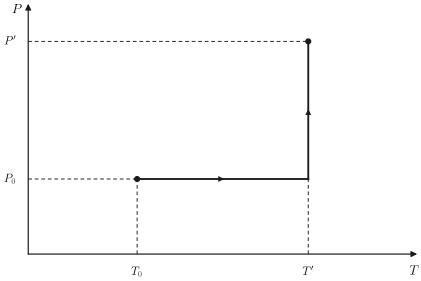
PROBLEMS
3.9-1.
- Show that for the multicomponent simple ideal gas \[ \begin{aligned} c_{v} & =\bar{c} R \\ \alpha & =1 / T \\ \kappa_{T} & =1 / P \end{aligned} \]
and
\[ \begin{aligned} & \kappa_{S}=\frac{\bar{c}}{\bar{c}+1} \frac{1}{P} \\ & c_{P}=(\bar{c}+1) R \quad \text { where } \bar{c}=\sum_{j} c_{j} x_{j}=\frac{1}{N} \sum_{j} c_{j} N_{j} \end{aligned} \]
What is the value of \(\bar{c}\) for a monatomic ideal gas?
Using the values found in part (a), corroborate equations 3.75 and 3.76.
Problem 3.9-2
Corroborate equation 3.70 for a multicomponent simple ideal gas, showing that both the right- and left-hand members of the equation equal \(-T / \bar{c} V\) (where \(\bar{c}\) is defined in Problem 3.9-1).
Problem 3.9-3
Compute the coefficient of expansion \(\alpha\) and the isothermal compressibility \(\kappa_{T}\) in terms of \(P\) and \(v\) for a system with the van der Waals equation of state (equation 3.41).
Problem 3.9-4
Compute \(c_{P}, c_{v}, \kappa_{S}\), and \(\kappa_{T}\) for the system in Problem 1.10-1(a). With these values corroborate the validity of equations 3.75 and 3.76.
Problem 3.9-5
From equations 3.75 and 3.76 show that
\[ c_{P} / c_{v}=\kappa_{T} / \kappa_{S} \]
Problem 3.9-6
A simple fundamental equation that exhibits some of the qualitative properties of typical crystaline solids is
\[ u=A e^{b\left(v-v_{0}\right)^{2}} s^{4 / 3} e^{s / 3 R} \]
where \(A, b\), and \(v_{0}\) are positive constants.
Show that the system satisfies the Nernst theorem.
Show that \(c_{v}\) is proportional to \(T^{3}\) at low temperature. This is commonly observed (and was explained by P. Debye by a statistical mechanical analysis, which will be developed in Chapter 16).
Show that \(c_{v} \rightarrow 3 k_{B}\) at high temperatures. This is the “equipartition value,” which is observed and which will be demonstrated by statistical mechanical analysis in Chapter 16.
Show that for zero pressure the coefficient of thermal expansion vanishes in this model-a result that is incorrect. Hint: Calculate the value of \(v\) at \(P=0\).
Problem 3.9-7
The density of mercury at various temperatures is given here in grams/ \(\mathrm{cm}^{3}\).
| \(13.6202\left(-10^{\circ} \mathrm{C}\right)\) | \(13.5217\left(30^{\circ} \mathrm{C}\right)\) | \(13.3283\left(110^{\circ} \mathrm{C}\right)\) |
|---|---|---|
| 13.5955 (0°C) | \(13.4973\left(40^{\circ} \mathrm{C}\right)\) | \(13.1148\left(200^{\circ} \mathrm{C}\right)\) |
| \(13.5708\left(10^{\circ} \mathrm{C}\right)\) | \(13.4729\left(50^{\circ} \mathrm{C}\right)\) | \(12.8806\left(300^{\circ} \mathrm{C}\right)\) |
| \(13.5462\left(20^{\circ} \mathrm{C}\right)\) | \(13.3522\left(100^{\circ} \mathrm{C}\right)\) | \(12.8572\left(310^{\circ} \mathrm{C}\right)\) |
Calculate \(\alpha\) at \(0^{\circ} \mathrm{C}\), at \(45^{\circ} \mathrm{C}\), at \(105^{\circ} \mathrm{C}\), and at \(305^{\circ} \mathrm{C}\). Should the stem of a mercury-in-glass thermometer be marked off in equal divisions for equal temperature intervals if the coefficient of th nal expansion of glass is assumed to be strictly constant?
Problem 3.9-8
For a particular material \(c_{P}, \alpha\), and \(\kappa_{T}\) can be represented empirically by power series in the vicinity of \(T_{0}, P_{0}\), as follows
\[ \begin{aligned} & c_{P}=c_{P}^{0}+A_{c} \tau+B_{c} \tau^{2}+D_{c} p+E_{c} p^{2}+F_{c} \tau p \\ & \alpha=\alpha^{0}+A_{\alpha} \tau+B_{\alpha} \tau^{2}+D_{\alpha} p+E_{\alpha} p^{2}+F_{\alpha} \tau p \\ & \kappa_{T}=\kappa^{0}+A_{\kappa} \tau+B_{\kappa} \tau^{2}+D_{\kappa} p+E_{\kappa} p^{2}+F_{\kappa} \tau p \quad \text { where } \tau \equiv T-T_{0} ; p \equiv P-P_{0} \end{aligned} \]
Find the molar volume explicitly as a function of \(T\) and \(P\) in the vicinity of ( \(T_{0}, P_{0}\) ).
Problem 3.9-9
Calculate the molar entropy \(s\left(T, P_{0}\right)\) for fixed pressure \(P_{0}\) and for temperature \(T\) in the vicinity of \(T_{0}\). Assume that \(c_{p}, \alpha\), and \(\kappa_{T}\) are given in the vicinity of ( \(T_{0}, P_{0}\) ) as in the preceding problem, and assume that \(s\left(T_{0}, P_{0}\right)\) is known.
Problem 3.9-10
By analogy with equations 3.70 and 3.71 show that for a paramagnetic system
\[ \left(\frac{\partial B_{e}}{\partial S}\right)_{I, V, N}=\left(\frac{\partial T}{\partial I}\right)_{S, V, N} \]
or, inverting,
\[ T\left(\frac{\partial S}{\partial B_{e}}\right)_{I, V, N}=T\left(\frac{\partial I}{\partial T}\right)_{S, V, N} \]
Interpret the physical meaning of this relationship.
Problem 3.9-11
By analogy with equations 3.70 and 3.71 show that for a paramagnetic system
\[ \left(\frac{\partial B_{e}}{\partial V}\right)_{S, I, N}=-\left(\frac{\partial P}{\partial I}\right)_{S, V, N} \]
Problem 3.9-12
The magnetic analogues of the molar heat capacities \(c_{P}\) and \(c_{v}\) are \(c_{B}\) and \(c_{I}\). Calculate \(c_{B}\left(T, B_{e}, N\right)\) and \(c_{I}\left(T, B_{e}, N\right)\) for the paramagnetic model of equation 3.66. (Note that no distinction need be made between \(c_{I, V}\) and \(c_{I, P}\) for this model, because of the absence of a dependence on volume in the fundamental relation (3.66). Generally all four heat capacities exist and are distinct.)
Problem 3.9-13
The (isothermal) molar magnetic susceptibility is defined by
\[ \chi \equiv \frac{\mu_{0}}{N}\left(\frac{\partial I}{\partial B_{e}}\right)_{T} \]
Show that the susceptibility of the paramagnetic model of equation 3.66 varies inversely with the temperature, and evaluate \(\chi_{1}\), defined as the value of \(\chi\) for \(T=1 \mathrm{~K}\).
Problem 3.9-14
Calculate the adiabatic molar susceptibility
\[ \chi_{s} \equiv \frac{\mu_{0}}{N}\left(\frac{\partial I}{\partial B_{e}}\right)_{S} \]
as a function of \(T\) and \(B_{e}\) for ..e paramagnetic model of equation 3.66.
Problem 3.9-15
Calculate the isothermal and adia…ic molar susceptibilities (defined in Problems 3.9-13 and 3.9-14) for the system with fundamental equation
\[ U=\frac{\mu_{0}}{2} \frac{I^{2}}{N_{\chi}}+N \varepsilon \exp (2 S / N R) \]
How are each of these related to the constant ” \(\chi\) ” appearing in the fundamental relation?
Problem 3.9-16
Show that for the system of Problem 3.8-2
\[ \left(\frac{\partial T}{\partial B_{e}}\right)_{S}=\left(\frac{\partial T}{\partial I}\right)_{S}=\left(\frac{\partial S}{\partial I}\right)_{T}=\left(\frac{\partial S}{\partial B_{e}}\right)_{T}=0 \]
and
\[ \left(\frac{\partial B_{e}}{\partial T}\right)_{I}=\left(\frac{\partial B_{e}}{\partial S}\right)_{I}=\left(\frac{\partial I}{\partial T}\right)_{B_{e}}=\left(\frac{\partial I}{\partial S}\right)_{B_{e}}=0 \]
That is, there is no “coupling” between the thermal and magnetic properties. What is the (atypical) feature of the equation of state of this system that leads to these results?
Problem 3.9-17
Calculate the heat transfer to a particular system if 1 mole is taken from \(\left(T_{0}, P_{0}\right)\) to \(\left(2 T_{0}, 2 P_{0}\right)\) along a straight line in the \(T-P\) plane. For this system it is known that:
\[ \begin{aligned} \alpha(T, P) & =\alpha^{0} \cdot\left(\frac{T}{T_{0}}\right)^{\frac{1}{2}}, \text { where } \alpha^{0} \text { is a constant } \\ c_{P}(T, P) & =c_{P}^{0}, \text { a constant } \\ \kappa_{T}(T, P) & =\kappa_{T}^{0}, \text { a constant } \end{aligned} \]
Hint: Use the relation \((\partial s / \partial P)_{T}=-(\partial v / \partial T)_{P}\), analogous to equations 3.70 through 3.72 (and to be derived systematically in Chapter 7), to establish that \(d Q=T d s=c_{P} d T-T v \alpha d P\).