THE CONDITIONS OF EQUILIBRIUM
2-1 INTENSIVE PARAMETERS
By virtue of our interest in processes, and in the associated changes of the extensive parameters, we anticipate that we shall be concerned with the differential form of the fundamental equation. Writing the fundamental equation in the form
\[ U=U\left(S, V, N_{1}, N_{2}, \ldots, N_{r}\right) \]
we compute the first differential:
\[ d U=\left(\frac{\partial U}{\partial S}\right)_{V, N_{1}, \ldots, N_{r}} d S+\left(\frac{\partial U}{\partial V}\right)_{S, N_{1}, \ldots, N_{r}} d V+\sum_{j=1}^{r}\left(\frac{\partial U}{\partial N_{j}}\right)_{S, V_{\ldots}, N_{r}} d N_{j} \]
The various partial derivatives appearing in the foregoing equation recur so frequently that it is convenient to introduce special symbols for them. They are called intensive parameters, and the following notation is conventional:
\[ \begin{aligned} \left(\frac{\partial U}{\partial S}\right)_{V, N_{1} \ldots, N_{r}} & \equiv T, \text { the temperature } \\ -\left(\frac{\partial U}{\partial V}\right)_{S, N_{1} \ldots, N_{r}} & \equiv P, \text { the pressure } \\ \left(\frac{\partial U}{\partial N_{j}}\right)_{S, V_{\ldots} \ldots N_{k} \ldots} & \equiv \mu_{j}, \text { the electrochemical potential of } \end{aligned} \]
With this notation, equation 2.2 becomes
\[ d U=T d S-P d V+\mu_{1} d N_{1}+\cdots+\mu_{r} d N_{r} \]
The formal definition of the temperature soon will be shown to agree with our intuitive qualitative concept, based on the physiological sensations of “hot” and “cold.” We certainly would be reluctant to adopt a definition of the temperature that would contradict such strongly entrenched although qualitative notions. For the moment, however, we merely introduce the concept of temperature by the formal definition (2.3).
Similarly, we shall soon corroborate that the pressure defined by equation 2.4 agrees in every respect with the pressure defined in mechanics. With respect to the several electrochemical potentials, we have no prior definitions or concepts and we are free to adopt the definition (equation 2.5) forthwith.
For brevity, the electrochemical potential is often referred to simply as the chemical potential, and we shall use these two terms interchangeably \({ }^{1}\).
The term \(-P d V\) in equation 2.6 is identified as the quasi-static work \(d W_{M}\), as given by equation 1.1.
In the special case of constant mole numbers equation 2.6 can then be written as
\[ T d S=d U-d W_{M} \quad \text { if } \quad d N_{1}=d N_{2}=d N_{r}=0 \]
Recalling the definition of the quasi-static heat, or comparing equation 2.7 with equation 1.2, we now recognize \(T d S\) as the quasi-static heat flux.
\[ d Q=T d S \]
A quasi-static flux of heat into a system is associated with an increase of entropy of that system.
The remaining terms in equation 2.6 represent an increase of internal energy associated with the addition of matter to a system. This type of energy flux, although intuitively meaningful, is not frequently discussed outside thermodynamics and does not have a familiar distinctive name. We shall call \(\Sigma_{j} \mu_{j} d N_{j}\) the quasi-static chemical work.
\[ d W_{c} \equiv \sum_{j=1}^{r} \mu_{j} d N_{j} \]
[^6]Therefore
\[ d U=d Q+d W_{M}+d W_{c} \]
Each of the terms \(T d S,-P d V, \mu_{J} d N_{J}\), in equation 2.6 has the dimensions of energy. The matter of units will be considered in Section 2.6. We can observe here, however, that having not yet specified the units (nor even the dimensions) of entropy, the units and dimensions of temperature remain similarly undetermined. The units of \(\mu\) are the same as those of energy (as the mole numbers are dimensionless). The units of pressure are familiar, and conversion factors are listed inside the back cover of this book.
2-2 EQUATIONS OF STATE
The temperature, pressure, and electrochemical potentials are partial derivatives of functions of \(S, V, N_{1}, \ldots, N_{r}\) and consequently are also functions of \(S, V, N_{1}, \ldots, N_{r}\). We thus have a set of functional relationships
\[ \begin{aligned} \frac{\partial u / s,}{\partial}= & T=T\left(S, V, N_{1}, \ldots, N_{r}\right) \\ & P=P\left(S, V, N_{1}, \ldots, N_{r}\right) \\ \frac{\partial}{\partial t} & \mu_{j}=\mu_{j}\left(S, V, N_{1}, \ldots, N_{r}\right) \end{aligned} \]
Such relationships, expressing intensive parameters in terms of the independent extensive parameters, are called equations of state.
Knowledge of a single equation of state does not constitute complete knowledge of the thermodynamic properties of a system. We shall see, subsequently, that knowledge of all the equations of state of a system is equivalent to knowledge of the fundamental equation and consequently is thermodynamically complete.
The fact that the fundamental equation must be homogeneous first order has direct implications for the functional form of the equations of state. It follows immediately that the equations of state are homogeneous zero order. That is, multiplication of each of the independent extensive parameters by a scalar \(\lambda\) leaves the function unchanged.
\[ T\left(\lambda S, \lambda V, \lambda_{1}, \ldots, \lambda N_{r}\right)=T\left(S, V, N_{1}, \ldots, N_{r}\right) \]
It therefore follows that the temperature of a portion of a system is equal to the temperature of the whole system. This is certainly in agreement with the intuitive concept of temperature. The pressure and the electrochemical potentials also have the property (2.14), and together with the temperature are said to be intensive.
To summarize the foregoing considerations it is convenient to adopt a condensed notation. We denote the extensive parameters \(V, N_{1}, \ldots, N_{r}\) by the symbols \(X_{1}, X_{2}, \ldots, X_{t}\), so that the fundamental relation takes the form
\[ U=U\left(S, X_{1}, X_{2}, \ldots, X_{t}\right) \]
The intensive parameters are denoted by
\[ \begin{aligned} \left(\frac{\partial U}{\partial S}\right)_{X_{1}, X_{2}, \ldots} & \equiv T=T\left(S, X_{1}, X_{2}, \ldots, X_{t}\right) \\ \left(\frac{\partial U}{\partial X_{j}}\right)_{S, \ldots, X_{k}, \ldots} & \equiv P_{j}=P_{j}\left(S, X_{1}, X_{2}, \ldots, X_{t}\right) \quad j=1,2, \ldots, t \end{aligned} \]
whence
\[ d U=T d S+\sum_{j=1}^{t} P_{j} d X_{j} \]
It should be noted that a negative sign appears in equation 2.4, but does not appear in equation 2.17. The formalism of thermodynamics is uniform if the negative pressure, \(-P\), is considered as an intensive parameter analogous to \(T\) and \(\mu_{1}, \mu_{2}, \ldots\). Correspondingly one of the general intensive parameters \(P_{j}\) of equation 2.17 is \(-P\).
For single-component simple systems the energy differential is frequently written in terms of molar quantities. Analogous to equations 1.11 through 1.15, the fundamental equation per mole is
\[ u=u(s, v) \]
where
\[ s=S / N, \quad v=V / N \]
and
\[ u(s, v)=\frac{1}{N} U(S, V, N) \]
Taking an infinitesimal variation of equation 2.19
\[ d u=\frac{\partial u}{\partial s} d s+\frac{\partial u}{\partial v} d v \]
However
\[ \left(\frac{\partial u}{\partial s}\right)_{v}=\left(\frac{\partial u}{\partial s}\right)_{V, N}=\left(\frac{\partial U}{\partial S}\right)_{V, N}=T \]
and similarly
\[ \left(\frac{\partial u}{\partial v}\right)_{s}=-P \]
Thus
\[ d u=T d s-P d v \]
PROBLEMS
Problem 2.2-1
Find the three equations of state for a system with the fundamental equation
\[ U=\left(\frac{v_{0} \theta}{R^{2}}\right) \frac{S^{3}}{N V} \]
Corroborate that the equations of state are homogeneous zero order (i.e., that \(T\), \(P\), and \(\mu\) are intensive parameters).
Problem 2.2-2
For the system of problem 2.2-1 find \(\mu\) as a function of \(T, V\), and \(N\).
Problem 2.2-3
Show by a diagram (drawn to arbitrary scale) the dependence of pressure on volume for fixed temperature for the system of problem 2.2-1. Draw two such “isotherms,” corresponding to two values of the temperature, and indicate which isotherm corresponds to the higher temperature.
Problem 2.2-4
Find the three equations of state for a system with the fundamental equation
\[ u=\left(\frac{\theta}{R}\right) s^{2}-\left(\frac{R \theta}{v_{0}^{2}}\right) v^{2} \]
and show that, for this system, \(\mu=-u\).
Problem 2.2-5
Express \(\mu\) as a function of \(\boldsymbol{T}\) and \(\boldsymbol{P}\) for the system of problem 2.2-4.
Problem 2.2-6
Find the three equations of state for a system with the fundamental equation
\[ u=\left(\frac{v_{0} \theta}{R}\right) \frac{s^{2}}{v} e^{s / R} \]
Problem 2.2-7
A particular system obeys the relation
\[ u=A v^{-2} \exp (s / R) \]
\(N\) moles of this substance, initially at temperature \(T_{0}\) and pressure \(P_{0}\), are expanded isentropically \((s=\) constant \()\) until the pressure is halved. What is the final temperature?
Answer:
\[ T_{f}=0.63 T_{0} \]
Problem 2.2-8
Show that, in analogy with equation 2.25 , for a system with \(r\) components
\[ d u=T d s-P d v+\sum_{j=1}^{r-1}\left(\mu_{j}-\mu_{r}\right) d x_{j} \]
where the \(x_{j}\) are the mole fractions \(\left(=N_{j} / N\right)\).
Problem 2.2-9
Show that if a single-component system is such that \(P V^{k}\) is constant in an adiabatic process ( \(k\) is a positive constant) the energy is
\[ U=\frac{1}{k-1} P V+N f\left(P V^{k} / N^{k}\right) \]
where \(f\) is an arbitrary function. Hint: \(P V^{k}\) must be a function of \(S\), so that \((\partial U / \partial V)_{S}=g(S) \cdot V^{-h}\), where \(g(S)\) is an unspecified function.
2-3 ENTROPIC INTENSIVE PARAMETERS
If, instead of considering the fundamental equation in the form \(U=\) \(U\left(S, \ldots, X_{j}, \ldots\right)\) with \(U\) as dependent, we had considered \(S\) as dependent, we could have carried out all the foregoing formalism in an inverted but equivalent fashion. Adopting the notation \(X_{0}\) for \(U\), we write
\[ S=S\left(X_{0}, X_{1}, \ldots, X_{l}\right) \]
We take an infinitesimal variation to obtain
\[ d S=\sum_{k=0}^{t} \frac{\partial S}{\partial X_{k}} d X_{k} \]
The quantities \(\partial S / \partial X_{k}\) are denoted by \(F_{k}\).
\[ F_{k} \equiv \frac{\partial S}{\partial X_{k}} \]
By carefully noting which variables are kept constant in the various partial derivatives (and by using the calculus of partial derivatives as reviewed in Appendix A) the reader can demonstrate that
\[ F_{0}=\frac{1}{T}, \quad F_{k}=\frac{-P_{k}}{T} \quad(k=1,2,3, \ldots) \]
These equations also follow from solving equation 2.18 for \(d S\) and comparing with equation 2.27.
Despite the close relationship between the \(F_{k}\) and the \(P_{k}\), there is a very important difference in principle. Namely, the \(P_{k}\) are obtained by differentiating a function of \(S, \ldots, X_{J}, \ldots\) and are considered as functions of these variables, whereas the \(F_{k}\) are obtained by differentiating a function of \(U, \ldots, X, \ldots\) and are considered as functions of these latter variables. That is, in one case the entropy is a member of the set of independent parameters, and in the second case the energy is such a member. In performing formal manipulations in thermodynamics it is extremely important to make a definite commitment to one or the other of these choices and to adhere rigorously to that choice. A great deal of confusion results from a vacillation between these two alternatives within a single problem.
If the entropy is considered dependent and the energy independent, as in \(S=S\left(U, \ldots, X_{k}, \ldots\right)\), we shall refer to the analysis as being in the entropy representation. If the energy is dependent and the entropy is independent, as in \(U=U\left(S, \ldots, X_{k}, \ldots\right)\), we shall refer to the analysis as being in the energy representation.
The formal development of thermodynamics can be carried out in either the energy or entropy representations alone, but for the solution of a particular problem either one or the other representation may prove to be by far the more convenient. Accordingly, we shall develop the two representations in parallel, although a discussion presented in one representation generally requires only a brief outline in the alternate representation.
The relation \(S=S\left(X_{0}, \ldots, X_{j}, \ldots\right)\) is said to be the entropic fundamental relation, the set of variables \(X_{0}, \ldots, X_{j}, \ldots\) is called the entropic extensive parameters, and the set of variables \(F_{0}, \ldots, F_{j}, \ldots\) is called the entropic intensive parameters. Similarly, the relation \(U=U\left(S, X_{1}\right.\) \(\left., \ldots, X_{j}, \ldots\right)\) is said to be the energetic fundamental relation; the set of variables \(S, X_{1}, \ldots, X_{1}, \ldots\) is called the energetic extensive parameters; and the set of variables \(T, P_{1}, \ldots, P_{j}, \ldots\) is called the energetic intensive parameters.
PROBLEMS
Problem 2.3-1
Find the three equations of state in the entropy representation for a system with the fundamental equation
\[ u=\left(\frac{v_{0}^{1 / 2} \theta}{R^{3 / 2}}\right) \frac{s^{5 / 2}}{v^{1 / 2}} \]
Answer:
\[ \begin{array}{r} \frac{1}{T}=\frac{2}{5}\left(\frac{v_{0}^{1 / 2} \theta}{R^{3 / 2}}\right)^{-2 / 5} \frac{v^{1 / 5}}{u^{3 / 5}} \\ \frac{\mu}{T}=-\frac{2}{5}\left(\frac{v_{0}^{1 / 2} \theta}{R^{3 / 2}}\right)^{-2 / 5} u^{2 / 5} v^{1 / 5} \end{array} \]
Problem 2.3-2
Show by a diagram (drawn to arbitrary scale) the dependence of tempera ture on volume for fixed pressure for the system of problem 2.3-1. Draw two such “isobars” corresponding to two values of the pressure, and indicate which isobar corresponds to the higher pressure.
Problem 2.3-3
Find the three equations of state in the entropy representation for a system with the fundamental equation
\[ u=\left(\frac{\theta}{R}\right) s^{2} e^{-v^{2} / v_{0}^{2}} \]
Problem 2.3-4
Consider the fundamental equation
\[ S=A U^{n} V^{m} N^{r} \]
where \(A\) is a positive constant. Evaluate the permissible values of the three constants \(n, m\), and \(r\) if the fundamental equation is to satisfy the thermodynamic postulates and if, in addition, we wish to have \(P\) increase with \(U / V\), at constant \(N\). (This latter condition is an intuitive substitute for stability requirements to be studied in Chapter 8.) For definiteness, the zero of energy is to be taken as the energy of the zero-temperature state.
Problem 2.3-5
Find the three equations of state for a system with the fundamental relation
\[ \frac{S}{R}=\frac{U V}{N}-\frac{N^{3}}{U V} \]
Show that the equations of state in entropy representation are homogeneous zero-order functions.
Show that the temperature is intrinsically positive.
Find the “mechanical equation of state” \(P=P(T, v)\).
Find the form of the adiabats in the \(P-v\) plane. (An “adiabat” is a locus of constant entropy, or an “isentrope”).
2-4 THERMAL EQUILIBRIUM-TEMPERATURE
We are now in a position to illustrate several interesting implications of the extremum principle which has been postulated for the entropy. Consider a closed composite system consisting of two simple systems separated by a wall that is rigid and impermeable to matter but that does allow the flow of heat. The volumes and mole numbers of each of the simple systems are fixed, but the energies \(U^{(1)}\) and \(U^{(2)}\) are free to change, subject to the conservation restriction
\[ U^{(1)}+U^{(2)}=\text { constant } \]
imposed by the closure of the composite system as a whole. Assuming that the system has come to equilibrium, we seek the values of \(U^{(1)}\) and \(U^{(2)}\). According to the fundamental postulate, the values of \(U^{(1)}\) and \(U^{(2)}\) are such as to maximize the entropy. Therefore, by the usual mathematical condition for an extremum, it follows that in the equilibrium state a virtual infinitesimal transfer of energy from system 1 to system 2 will produce no change in the entropy of the whole system. That is,
\[ d S=0 \]
The additivity of the entropy for the two subsystems gives the relation
\[ S=S^{(1)}\left(U^{(1)}, V^{(1)}, \ldots, N_{j}^{(1)}, \ldots\right)+S^{(2)}\left(U^{(2)}, V^{(2)}, \ldots, N_{j}^{(2)}, \ldots\right) . \]
As \(U^{(1)}\) and \(U^{(2)}\) are changed by the virtual energy transfer, the entropy change is
\[ d S=\left(\frac{\partial S^{(1)}}{\partial U^{(1)}}\right)_{V^{(1)}, \ldots, N_{j}^{(1)}, \ldots} d U^{(1)}+\left(\frac{\partial S^{(2)}}{\partial U^{(2)}}\right)_{V^{(2)}, \ldots, N_{j}^{(2)}, \ldots} d U^{(2)} \]
or, employing the definition of the temperature
\[ d S=\frac{1}{T^{(1)}} d U^{(1)}+\frac{1}{T^{(2)}} d U^{(2)} \]
By the conservation condition (equation 2.30), we have
\[ d U^{(2)}=-d U^{(1)} \]
whence
\[ d S=\left(\frac{1}{T^{(1)}}-\frac{1}{T^{(2)}}\right) d U^{(1)} \]
The condition of equilibrium (equation 2.31) demands that \(d S\) vanish for arbitrary values of \(d U^{(1)}\), whence
\[ \frac{1}{T^{(1)}}=\frac{1}{T^{(2)}} \]
This is the condition of equilibrium. If the fundamental equations of each of the subsystems were known, then \(1 / T^{(1)}\) would be a known function of \(U^{(1)}\) (and of \(V^{(1)}\) and \(N_{k}^{(1)}, \ldots\), which, however, are merely constants). Similarly, \(1 / T^{(2)}\) would be a known function of \(U^{(2)}\), and the equation \(1 / T^{(1)}=1 / T^{(2)}\) would be one equation in \(U^{(1)}\) and \(U^{(2)}\). The conservation condition \(U^{(1)}+U^{(2)}=\) constant provides a second equation, and these two equations completely determine, in principle, the values of \(U^{(1)}\) and of \(U^{(2)}\). To proceed further and actually to obtain the values of \(U^{(1)}\) and \(U^{(2)}\) would require knowledge of the explicit forms of the fundamental equations of the systems. In thermodynamic theory, however, we accept the existence of the fundamental equations, but we do not assume explicit forms for them, and we therefore do not obtain explicit answers. In practical applications of thermodynamics the fundamental equations may be known, either by empirical observations (in terms of measurements to be described later) or on the basis of statistical mechanical calculations based on simple models. In this way applied thermodynamics is able to lead to explicit numerical answers.
Equation 2.37 could also be written as \(T^{(1)}=T^{(2)}\). We write it in the form \(1 / T^{(1)}=1 / T^{(2)}\) to stress the fact that the analysis is couched in the entropy representation. By writing \(1 / T^{(1)}\), we indicate a function of \(U^{(1)}, V^{(1)}, \ldots\), whereas \(T^{(1)}\) would imply a function of \(S^{(1)}, V^{(1)}, \ldots\). The physical significance of equation 2.37, however, remains the equality of the temperatures of the two subsystems.
A second phase of the problem is the investigation of the stability of the predicted final state. In the solution given we have not exploited fully the basic postulate that the entropy is a maximum in equilibrium; rather, we merely have investigated the consequences of the fact that it is an extremum. The condition that it be a maximum requires, in addition to the condition \(d S=0\), that
\[ d^{2} S<0 \]
The consequences of this condition lead to considerations of stability, to which we shall give explicit attention in Chapter 8.
2-5 AGREEMENT WITH INTUITIVE CONCEPT OF TEMPERATURE
In the foregoing example we have seen that if two systems are separated by a diathermal wall, heat will flow until each of the system attains the same temperature. This prediction is in agreement with our intuitive notion of temperature, and it is the first of several observations that corroborate the plausibility of the formal definition of the temperature.
Inquiring into the example in slightly more detail, we suppose that the two subsystems initially are separated by an adiabatic wall and that the temperatures of the two subsystems are almost, but not quite, equal. In particular we assume that
\[ T^{(1)}>T^{(2)} \]
The system is considered initially to be in equilibrium with respect to the internal adiabatic constraint. If the internal adiabatic constraint now is removed, the system is no longer in equilibrium, heat flows across the wall, and the entropy of the composite system increases. Finally the system comes to a new equilibrium state, determined by the condition that the final values of \(T^{(1)}\) and \(T^{(2)}\) are equal, and with the maximum possible value of the entropy that is consistent with the remaining constraints. Compare the initial and the final states. If \(\Delta S\) denotes the entropy difference between the final and initial states
\[ \Delta S>0 \]
But, as in equation 2.36,
\[ \Delta S \simeq\left(\frac{1}{T^{(1)}}-\frac{1}{T^{(2)}}\right) \Delta U^{(1)} \]
where \(T^{(1)}\) and \(T^{(2)}\) are the initial values of the temperatures. By the condition that \(T^{(1)}>T^{(2)}\), it follows that
\[ \Delta U^{(1)}<0 \]
This means that the spontaneous process that occurred was one in which heat flowed from subsystem 1 to subsystem 2 . We conclude therefore that heat tends to flow from a system with a high value of \(T\) to a system with a low value of \(T\). This is again in agreement with the intuitive notion of temperature. It should be noted that these conclusions do not depend on the assumption that \(T^{(1)}\) is approximately equal to \(T^{(2)}\); this assumption was made merely for the purpose of obtaining mathematical simplicity in equation 2.41 , which otherwise would require a formulation in terms of
If we now take stock of our intuitive notion of temperature, based on integrals. the physiological sensations of hot and cold, we realize that it is based upon two essential properties. First, we expect temperature to be an intensive parameter, having the same value in a part of a system as it has in the entire system. Second, we expect that heat should tend to flow from regions of high temperature toward regions of low temperature. These properties imply that thermal equilibrium is associated with equality and homogeneity of the temperature. Our formal definition of the temperature possesses each of these properties.
2-6 TEMPERATURE UNITS
The physical dimensions of temperature are those of energy divided by those of entropy. But we have not yet committed ourselves on the dimensions of entropy; in fact its dimensions can be selected quite arbitrarily. If the entropy is multiplied by any positive dimensional constant we obtain a new function of different dimensions but with exactly the same extremum properties-and therefore equally acceptable as the entropy. We summarily resolve the arbitrariness simply by adopting the convention that the entropy is dimensionless (from the more incisive viewpoint of statistical mechanics this is a physically reasonable choice). Consequently the dimensions of temperature are identical to those of energy. However, just as torque and work have the same dimensions, but are different types of quantities and are measured in different units (the meter-Newton and the joule, respectively), so the temperature and the energy should be carefully distinguished. The dimensions of both energy and temperature are [mass . (length) \({ }^{2}\) /(time) \({ }^{2}\) ]. The units of energy are joules, ergs, calories, and the like. The units of temperature remain to be
In our later discussion of thermodynamic “Carnot” engines, in Chapter discussed. 4, we shall find that the optimum performance of an engine in contact with two thermodynamic systems is completely determined by the ratio of the temperatures of those two systems. That is, the principles of thermodynamics provide an experimental procedure that unambiguously determines the ratio of the temperatures of any two given systems.
The fact that the ratio of temperatures is measurable has immediate consequences. First the zero of temperature is uniquely determined and cannot be arbitrarily assigned or “shifted.” Second we are free to assign the value of unity (or some other value) to one arbitrary chosen state. All other temperatures are thereby determined.
Equivalently, the single arbitrary aspect of the temperature scale is the size of the temperature unit, determined by assigning a specific temperature to some particular state of a standard system.
The assignment of different temperature values to standard states leads to different thermodynamic temperature scales, but all thermodynamic temperature scales coincide at \(T=0\). Furthermore, according to equation 1.7 no system can have a temperature lower than zero. Needless to say, this essential positivity of the temperature is in full agreement with all measurements of thermodynamic temperatures.
The Kelvin scale of temperature, which is the official Système International (SI) system, is defined by assigning the number 273.16 to the temperature of a mixture of pure ice, water, and water vapor in mutual equilibrium; a state which we show in our later discussion of “triple points” determines a unique temperature. The corresponding unit of temperature is called a kelvin, designated by the notation \(K\).
The ratio of the kelvin and the joule, two units with the same dimensions, is \(1.3806 \times 10^{-23}\) joules/kelvin. This ratio is known as Boltzmann’s constant and is generally designated as \(k_{B}\). Thus \(k_{B} T\) is an energy.
The Rankine scale is obtained by assigning the temperature \(\left(\frac{9}{5}\right) \times\) \(273.16=491.688^{\circ} \mathrm{R}\) to the ice-water-water vapor system just referred to. The unit, denoted by \({ }^{\circ} \mathrm{R}\), is called the degree Rankine. Rankine temperatures are merely \(\frac{9}{5}\) times the corresponding Kelvin temperature.
Closely related to the “absolute” Kelvin scale of temperature is the International Kelvin scale, which is a “practical” scale, defined in terms of the properties of particular systems in various temperature ranges and contrived to coincide as closely as possible with the (absolute) Kelvin scale. The practical advantage of the International Kelvin scale is that it provides reproducible laboratory standards for temperature measurement throughout the temperature range. However, from the thermodynamic point of view, it is not a true temperature scale, and to the extent that it deviates from the absolute Kelvin scale it will not yield temperature ratios that are consistent with those demanded by the thermodynamic formalism.
The values of the temperature of everyday experiences are large numbers on both the Kelvin and the Rankine scales. Room temperatures are in the region of 300 K , or \(540^{\circ} \mathrm{R}\). For common usage, therefore, two derivative scales are in common use. The Celsius scale is defined as
\[ T\left({ }^{\circ} \mathrm{C}\right)=T(\mathrm{~K})-273.15 \]
where \(T\left({ }^{\circ} \mathrm{C}\right)\) denotes the “Celsius temperature,” for which the unit is called the degree Celsius, denoted by °C. The zero of this scale is displaced relative to the true zero of temperature, so the Celsius temperature scale is not a thermodynamic temperature scale at all. Negative temperatures appear, the zero is incorrect, and ratios of temperatures are not in agreement with thermodynamic principles. Only temperature differences are correctly given.
On the Celsius scale the “temperature” of the triple point (ice, water, and water vapor in mutual equilibrium) is \(0.01^{\circ} \mathrm{C}\). The Celsius temperature of an equilibrium mixture of ice and water, maintained at a pressure of 1 atm, is even closer to 0°C, with the difference appearing only in the third decimal place. Also the Celsius temperature of boiling water at 1 atm pressure is very nearly \(100^{\circ} \mathrm{C}\). These near equalities reveal the historical origin \({ }^{2}\) of the Celsius scale; before it was recognized that the zero of temperature is unique it was thought that two points, rather than one, could be arbitrarily assigned and these were taken (by Anders Celsius, in 1742) as the 0°C and 100°C just described.
The Fahrenheit scale is a similar “practical” scale. It is now defined by
\[ T\left({ }^{\circ} \mathrm{F}\right) \equiv T\left({ }^{\circ} \mathrm{R}\right)-459.67=\frac{9}{5} T\left({ }^{\circ} \mathrm{C}\right)+32 \]
The Fahrenheit temperature of ice and water at 1 atm pressure is roughly 32°F; the temperature of boiling water at 1 atm pressure is about 212°F; and room temperatures are in the vicinity of \(70^{\circ} \mathrm{F}\). More suggestive of the presumptive origins of this scale are the facts that ice, salt, and water coexist in equilibrium at 1 atm pressure at a temperature in the vicinity of \(0^{\circ} \mathrm{F}\), and that the body (i.e., rectal) temperature of a cow is roughly \(100^{\circ} \mathrm{F}\).
Although we have defined the temperature formally in terms of a partial derivative of the fundamental relation, we briefly note the conventional method of introduction of the temperature concept, as developed by Kelvin and Caratheodory. The heat flux \(d Q\) is first defined very much as we have introduced it in connection with the energy conservation principle. From the consideration of certain cyclic processes it is then inferred that there exists an integrating factor \((1 / T)\) such that the product of this integrating factor with the imperfect differential \(d Q\) is a perfect differential \((d S)\).
\[ d S=\frac{1}{T} d Q \]
[^7]The temperature and the entropy thereby are introduced by analysis of the existence of integrating factors in particular types of differential equations called Pfaffian forms.
PROBLEMS
Problem 2.6-1
The temperature of a system composed of ice, water, and water vapor in mutual equilibrium has a temperature of exactly 273.16 K, by definition. The temperature of a system of ice and water at 1 atm of pressure is then measured as 273.15 K, with the third and later decimal places uncertain. The temperature of a system of water and water vapor (i.e., boiling water) at 1 atm is measured as 373.15 K ± 0.01 K. Compute the temperature of water-water vapor at 1 atm, with its probable error, on the Celsius, absolute Fahrenheit, and Fahrenheit scales.
Problem 2.6-2
The “gas constant” \(R\) is defined as the product of Avogadro’s number ( \(N_{A}=6.0225 \times 10^{23} /\) mole ) and Boltzmann’s constant \(R \equiv N_{A} k_{B}\). Correspondingly \(R \simeq 8.314 \mathrm{~J} /\) mole K . Since the size of the Celsius degree is the same as the size of Kelvin degree, it has the value \(8.314 \mathrm{~J} /\) mole \(^{\circ} \mathrm{C}\). Express \(R\) in units of J/mole \({ }^{\circ} \mathrm{F}\).
Problem 2.6-3
Two particular systems have the following equations of state:
\[ \frac{1}{T^{(1)}}=\frac{3}{2} R \frac{N^{(1)}}{U^{(1)}} \]
and
\[ \frac{1}{T^{(2)}}=\frac{5}{2} R \frac{N^{(2)}}{U^{(2)}} \]
where \(R\) is the gas constant (Problem 2.6-2). The mole number of the first system is \(N^{(1)}=2\) and that of the second is \(N^{(2)}=3\). The two systems are separated by a diathermal wall, and the total energy in the composite system is \(2.5 \times 10^{3} \mathrm{~J}\). What is the internal energy of each system in equilibrium?
Answer:
\[ U^{(1)}=714.3 \mathrm{~J} \]
Problem 2.6-4
Two systems with the equations of state given in Problem 2.6-3 are separated by a diathermal wall. The respective mole numbers are \(N^{(1)}=2\) and \(N^{(2)}=3\). The initial temperatures are \(T^{(1)}=250 \mathrm{~K}\) and \(T^{(2)}=350 \mathrm{~K}\). What are the values of \(U^{(1)}\) and \(U^{(2)}\) after equilibrium has been established? What is the equilibrium temperature?
2-7 MECHANICAL EQUILIBRIUM
A second application of extremum principle for the entropy yields an even simpler result and ulerefore is useful in making the procedure clear. We consider a closed composite system consisting of two simple systems separated by a movable diathermal wall that is impervious to the flow of matter. The values of the mole numbers are fixed and constant, but the values of \(U^{(1)}\) and \(U^{(2)}\) can change, subject only to the closure condition
\[ U^{(1)}+U^{(2)}=\text { constant } \]
and the values of \(V^{(1)}\) and \(V^{(2)}\) can change, subject only to the closure condition
\[ V^{(1)}+V^{(2)}=\text { constant } \]
The extremum principle requires that no change in entropy result from infinitesimal virtual processes consisting of transfer of heat across the wall or of displacement of the wall.
Then
\[ d S=0 \]
where
\[ \begin{aligned} d S= & \left(\frac{\partial S^{(1)}}{\partial U^{(1)}}\right)_{V^{(1)}, \ldots N_{k}^{(1)}, \ldots} d U^{(1)}+\left(\frac{\partial S^{(1)}}{\partial V^{(1)}}\right)_{U^{(1)}, \ldots N_{k}^{(1)}, \ldots} d V^{(1)} \\ & +\left(\frac{\partial S^{(2)}}{\partial U^{(2)}}\right)_{V^{(2)}, \ldots N_{k}^{(2)}, \ldots} d U^{(2)}+\left(\frac{\partial S^{(2)}}{\partial V^{(2)}}\right)_{U^{(2)}, \ldots N_{k}^{(2)}, \ldots} d V^{(2)} \end{aligned} \]
By the closure conditions
\[ d U^{(2)}=-d U^{(1)} \]
and
\[ d V^{(2)}=-d V^{(1)} \]
whence
\[ d S=\left(\frac{1}{T^{(1)}}-\frac{1}{T^{(2)}}\right) d U^{(1)}+\left(\frac{P^{(1)}}{T^{(1)}}-\frac{P^{(2)}}{T^{(2)}}\right) d V^{(1)}=0 \]
As this expression must vanish for arbitrary and independent values of \(d U^{(1)}\) and \(d V^{(1)}\), we must have
\[ \frac{1}{T^{(1)}}-\frac{1}{T^{(2)}}=0 \]
and
\[ \frac{P^{(1)}}{T^{(1)}}-\frac{P^{(2)}}{T^{(2)}}=0 \]
Although these two equations are the equilibrium conditions in the proper form appropriate to the entropy representation, we note that they imply the physical conditions of equality of both temperature and pressure.
\[ \begin{aligned} & T^{(1)}=T^{(2)} \\ & P^{(1)}=P^{(2)} \end{aligned} \]
The equality of the temperatures is just our previous result for equilibrium with a diathermal wall. The equality of the pressures is the new feature introduced by the fact that the wall is movable. Of course, the equality of the pressures is precisely the result that we would expect on the basis of mechanics, and this result corroborates the identification of the function \(P\) as the mechanical pressure.
Again we stress that this result is a formal solution of the given problem. In the entropy representation, \(1 / T^{(1)}\) is a function of \(U^{(1)}, V^{(1)}\), and \(N^{(1)}\) (an entropic equation of state), so that equation 2.53 is formally a relationship among \(U^{(1)}, V^{(1)}, U^{(2)}\), and \(V^{(2)}\) (with \(N^{(1)}\) and \(N^{(2)}\) each held fixed). Similarly \(P^{(1)} / T^{(1)}\) is a function of \(U^{(1)}, V^{(1)}\), and \(N^{(1)}\), so that equation 2.54 is a second relationship among \(U^{(1)}, V^{(1)}, U^{(2)}\), and \(V^{(2)}\). The two conservation equations 2.46 and 2.47 complete the four equations required to determine the four sought-for variables. Again thermodynamics provides the methodology, which becomes explicit when applied to a concrete system with a definite fundamental relation, or with known equations of state.
The case of a moveable adiabatic (rather than diathermal) wall presents a unique problem with subtleties that are best discussed after the formalism is developed more fully; we shall return to that case in Problem 2.7-3 and in Problem 5.1-2.
Example 1
Three cylinders of identical cross-sectional areas are fitted with pistons, and each contains a gaseous system (not necessarily of the same composition). The pistons are connected to a rigid bar hinged on a fixed fulcrum, as indicated in Fig. 2.1. The “moment arms,” or the distances from the fulcrum, are in the ratio of 1 : 2 : 3. The cylinders rest on a heat conductive table of negligible mass; the table makes no contribution to the physics of the problem except to ensure that the three cylinders are in diathermal contact. The entire system is isolated and no pressure acts on the external surfaces of the pistons. Find the ratio of pressures and of temperatures in the three cylinders.
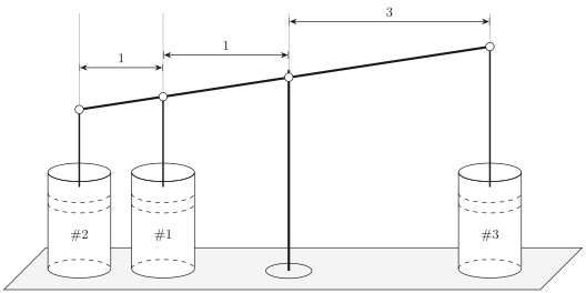
Solution The closure condition for the total energy is
\[ \delta U^{(1)}+\delta U^{(2)}+\delta U^{(3)}=0 \]
and the coupling of the pistons imposes the conditions that
\[ \delta V^{(2)}=2 \delta V^{(1)} \]
and
\[ \delta V^{(3)}=-3 \delta V^{(1)} \]
Then the extremal property of the entropy is
\[ \begin{aligned} \delta S= & \frac{1}{T^{(1)}} \delta U^{(1)}+\frac{1}{T^{(2)}} \delta U^{(2)}+\frac{1}{T^{(3)}} \delta U^{(3)}+\frac{P^{(1)}}{T^{(1)}} \delta V^{(1)} \\ & +\frac{P^{(2)}}{T^{(2)}} \delta V^{(2)}+\frac{P^{(3)}}{T^{(3)}} \delta V^{(3)}=0 \end{aligned} \]
Eliminating \(U^{(3)}, V^{(2)}\), and \(V^{(3)}\)
\[ \begin{aligned} \delta S= & \left(\frac{1}{T^{(1)}}-\frac{1}{T^{(3)}}\right) \delta U^{(1)}+\left(\frac{1}{T^{(2)}}-\frac{1}{T^{(3)}}\right) \delta U^{(2)} \\ & +\left(\frac{P^{(1)}}{T^{(1)}}+2 \frac{P^{(2)}}{T^{(2)}}-3 \frac{P^{(3)}}{T^{(3)}}\right) \delta V^{(1)}=0 \end{aligned} \]
The remaining three variations \(\delta U^{(1)}, \delta U^{(2)}\), and \(\delta V^{(1)}\) are arbitrary and unconstrained, so that the coefficient of each must vanish separately. From the coefficient of \(\delta U^{(1)}\) we find \(T^{(1)}=T^{(3)}\), and from the coefficient of \(\delta U^{(2)}\) we find \(T^{(2)}=T^{(3)}\). Hence all three systems come to a common final temperature. From the coefficient of \(\delta V^{(1)}\), and using the equality of the temperatures, we find
\[ P^{(1)}+2 P^{(2)}=3 P^{(3)} \]
This is the expected result, embodying the familiar mechanical principle of the lever. Explicit knowledge of the equations of state would ed le us to convert this into a solution for the volumes of the three systems.
PROBLEMS
Problem 2.7-1
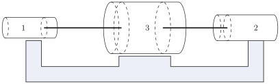
Three cylinders are fitted with four pistons, as shown in Fig. 2.2. The cross-sectional areas of the cylinders are in the ratio \(A_{1}: A_{2}: A_{3}=1: 2: 3\). Pairs of pistons are coupled so that their displacements (linear motions) are equal. The walls of the cylinders are diathermal and are connected by a heat conducting bar (crosshatched in the figure). The entire system is isolated (so that, for instance, there is no pressure exerted on the outer surfaces of the pistons). Find the ratios of pressures in the three cylinders.
Problem 2.7-2
Two particular systems have the following equations of state:
\[ \frac{1}{T^{(1)}}=\frac{3}{2} R \frac{N^{(1)}}{U^{(1)}}, \quad \frac{P^{(1)}}{T^{(1)}}=R \frac{N^{(1)}}{V^{(1)}} \]
and
\[ \frac{1}{T^{(2)}}=\frac{5}{2} R \frac{N^{(2)}}{U^{(2)}}, \quad \frac{P^{(2)}}{T^{(2)}}=R \frac{N^{(2)}}{V^{(2)}} \]
The mole number of the first system is \(N^{(1)}=0.5\) and that of the second is \(N^{(2)}=0.75\). The two systems are contained in a closed cylinder, separated by a fixed, adiabatic, and impermeable piston. The initial temperatures are \(T^{(1)}=200\) K and \(T^{(2)}=300 \mathrm{~K}\), and the total volume is 20 liters. The “setscrew” which prevents the motion of the piston is then removed, and simultaneously the adiabatic insulation of the piston is stripped off, so that the piston becomes moveable, diathermal, and impermeable. What is the energy, volume, pressure, and temperature of each subsystem when equilibrium is established?
It is sufficient to take \(R \simeq 8.3 \mathrm{~J} /\) mole K and to assume the external pressure to be zero.
\[ \begin{array}{r} \text { Answer: } \\ U^{(1)}=1700 \mathrm{~J} \end{array} \]
Problem 2.7-3
The hypothetical problem of equilibrium in a closed composite system with an internal moveable adiabatic wall is a unique indeterminate problem. Physically, release of the piston would lead it to perpetual oscillation in the absence of viscous damping. With viscou imping the piston would eventually come to rest at such a position that the pressures on either side would be equal, but the
temperatures in each subsystem would then depend on the relative viscosity in each subsystem. The solution of this problem depends on dynamical considerations. Show that the application of the entropy maximum formalism is correspondingly indeterminate with respect to the temperatures (but determinate with respect to the pressures). Hint: First show that with \(d U^{(1)}=-P^{(1)} d V^{(1)}\), and similarly for subsystem 2, energy conservation gives \(P^{(1)}=P^{(2)}\). Then show that the entropy maximum condition vanishes identically, giving no solution for \(T^{(1)}\) or \(T^{(2)}\).
2-8 EQUILIBRIUM WITH RESPECT TO MATTER FLOW
Consideration of the flow of matter provides insight into the nature of the chemical potential. We consider the equilibrium state of two simple systems connected by a rigid and diathermal wall, permeable to one type of material ( \(N_{1}\) ) and impermeable to all others ( \(N_{2}, N_{3}, \ldots, N_{r}\) ). We seek the equilibrium values of \(U^{(1)}\) and \(U^{(2)}\) and of \(N_{1}^{(1)}\) and \(N_{1}^{(2)}\). The virtual change in entropy in the appropriate virtual process is
\[ d S=\frac{1}{T^{(1)}} d U^{(1)}-\frac{\mu_{1}^{(1)}}{T^{(1)}} d N_{1}^{(1)}+\frac{1}{T^{(2)}} d U^{(2)}-\frac{\mu_{1}^{(2)}}{T^{(2)}} d N_{1}^{(2)} \]
and the closure conditions demand
\[ d U^{(2)}=-d U^{(1)} \]
and
\[ d N_{1}^{(2)}=-d N_{1}^{(1)} \]
whence
\[ d S=\left(\frac{1}{T^{(1)}}-\frac{1}{T^{(2)}}\right) d U^{(1)}-\left(\frac{\mu_{1}^{(1)}}{T^{(1)}}-\frac{\mu_{1}^{(2)}}{T^{(2)}}\right) d N_{1}^{(1)} \]
As \(d S\) must vanish for arbitrary values of both \(d U^{(1)}\) and \(d N_{1}^{(1)}\), we find as the conditions of equilibrium
\[ \frac{1}{T^{(1)}}=\frac{1}{T^{(2)}} \]
and
\[ \frac{\mu_{1}^{(1)}}{T^{(1)}}=\frac{\mu_{1}^{(2)}}{T^{(2)}} \quad\left(\text { hence also } \mu_{1}^{(1)}=\mu_{1}^{(2)}\right) \]
Thus, just as the temperature can be looked upon as a sort of “potential” for heat flux and the pressure can be looked upon as a sort of “potential” for volume changes, so the chemical potential can be looked upon as a sort of “potential” for matter flux. A difference in chemical potential provides a “generalized force” for matter flow.
The direction of the matter flow can be analyzed by the same method used in Section 2.5 to analyze the direction of the heat flow. If we assume that the temperatures \(T^{(1)}\) and \(T^{(2)}\) are equal, equation 2.60 becomes
\[ d S=\frac{\mu_{1}^{(2)}-\mu_{1}^{(1)}}{T} d N_{1}^{(1)} \]
If \(\mu_{1}^{(1)}\) is greater than \(\mu_{1}^{(2)}, d N_{1}^{(1)}\) will be negative, since \(d S\) must be positive. Thus matter tends to flow from regions of high chemical potential to regions of low chemical potential.
In later chapters we shall see that the chemical potential provides the generalized force not only for the flow of matter from point to point but also for its changes of phase and for chemical reactions. The chemical potential thus plays a dominant role in theoretical chemistry.
The units of chemical potential are joules per mole (or any desired energy unit per mole).
PROBLEMS
Problem 2.8-1
The fundamental equation of a particular type of two-component system is
\[ \begin{aligned} & S=N A+N R \ln \frac{U^{3 / 2} V}{N^{5 / 2}}-N_{1} R \ln \frac{N_{1}}{N}-N_{2} R \ln \frac{N_{2}}{N} \\ & N \equiv N_{1}+N_{2} \end{aligned} \]
where \(A\) is an unspecified constant. A closed rigid cylinder of total volume 10 liters is divided into two chambers of equal volume by a diathermal rigid membrane, permeable to the first component but impermeable to the second. In one chamber is placed a sample of the system with original parameters \(N_{1}^{(1)}=0.5\), \(N_{2}^{(1)}=0.75, V^{(1)}=5\) liters, and \(T^{(1)}=300 \mathrm{~K}\). In the second chamber is placed a sample with original parameters \(N_{1}^{(2)}=1, N_{2}^{(2)}=0.5, V^{(2)}=5\) liters, and \(T^{(2)}=\) 250 K. After equilibrium is established, what are the values of \(N_{1}^{(1)}, N_{1}^{(2)}, T, P^{(1)}\), and \(P^{(2)}\) ?
Answer:
\[ T=272.7 \mathrm{~K} \]
Problem 2.8-2
A two-component gaseous system has a fundamental equation of the form
\[ S=A U^{1 / 3} V^{1 / 3} N^{1 / 3}+\frac{B N_{1} N_{2}}{N}, \quad N=N_{1}+N_{2} \]
where \(A\) and \(B\) are positive constants. A closed cylinder of total volume \(2 V_{0}\) is separated into two equal subvolumes by a rigid diathermal partition permeable only to the first component. One mole of the first component, at a temperature \(T_{\ell}\), is introduced in the left-hand subvolume, and a mixture of \(\frac{1}{2}\) mole of each component, at a temperature \(T_{r}\), is introduced into the right-hand subvolume.
Find the equilibrium temperature \(T_{e}\) and the mole numbers in each subvolume when the system has come to equilibrium, assuming that \(T_{r}=2 T_{r}=400 \mathrm{~K}\) and that \(37 B^{2}=100 A^{3} V_{0}\). Neglect the heat capacity of the walls of the container!
Answer:
\[ N_{1 \ell}=0.9 \]
2-9 CHEMICAL EQUILIBRIUM
Systems that can undergo chemical reactions bear a strong formal similarity to the diffusional systems considered in the preceding section. Again they are governed by equilibrium conditions expressed in terms of the chemical potential \(\mu\)-whence derives its name chemical potential.
In a chemical reaction the mole numbers of the system change, some increasing at the expense of a decrease in others. The relationships among the changing mole numbers are governed by chemical reaction equations such as
\[ 2 \mathrm{H}_{2}+\mathrm{O}_{2} \rightleftharpoons 2 \mathrm{H}_{2} \mathrm{O} \]
or
\[ 2 \mathrm{O} \rightleftharpoons \mathrm{O}_{2} \]
The meaning of the first of these equations is that the changes in the mole numbers of hydrogen, oxygen, and water stand in the ratio of \(-2:-1:+2\). More generally one writes a chemical reaction equation, for a system with \(r\) components, in the form
\[ 0 \rightleftharpoons \sum_{j} \nu_{j} A_{j} \]
The \(\nu_{j}\) are the “stoichiometric coefficients” ( \(-2,-1,+2\) for the reaction of hydrogen and oxygen to form water), and the \(A_{j}\) are the symbols for the chemical components ( \(A_{1}=\mathrm{H}_{2}, A_{2}=\mathrm{O}_{2}\), and \(A_{3}=\mathrm{H}_{2} \mathrm{O}\) for the preceding reaction). If the reaction is viewed in the reverse sense (for instance, as the dissociation of water to hydrogen plus oxygen) the opposite signs would be assigned to each of the \(\nu_{j}\); this is a matter of arbitrary choice and only the relative signs of the \(\nu_{j}\) are significant.
The fundamental equation of the system is
\[ S=S\left(U, V, N_{1}, N_{2}, \ldots, N_{r}\right) \]
In the course of the chemical reaction both the total energy \(U\) and the total volume \(V\) remain fixed, the system being considered to be enclosed in an adiabatic and rigid “reaction vessel.” This is not the most common boundary condition for chemical reactions, which are more often carried out in open vessels, free to interchange energy and volume with the ambient atmosphere; we shall return to these open boundary conditions in Section 6.4. The change in entropy in a virtual chemical process is then
\[ d S=-\sum_{j=1}^{r} \frac{\mu_{j}}{T} d N_{j} \]
However, the changes in the mole numbers are proportional to the stoichiometric coefficients \(\nu_{j}\). Let the factor of proportionality be denoted by \(d \tilde{N}\), so that
\[ d S=-\frac{d \bar{N}}{T} \sum_{j=1}^{r} \mu_{j} \nu_{j} \]
Then the extremum principle dictates that, in equilibrium
\[ \sum_{j=1}^{r} \mu_{j} \nu_{j}=0 \]
If the equations of state of the mixture are known, the equilibrium condition (2.70) permits explicit solution for the final mole numbers.
It is of interest to examine this “solution in principle” in a slightly richer case. If hydrogen, oxygen, and carbon dioxide are introduced into a vessel the following chemical reactions may occur.
\[ \begin{aligned} \mathrm{H}_{2}+\frac{1}{2} \mathrm{O}_{2} & \rightleftharpoons \mathrm{H}_{2} \mathrm{O} \\ \mathrm{CO}_{2}+\mathrm{H}_{2} & \rightleftharpoons \mathrm{CO}+\mathrm{H}_{2} \mathrm{O} \\ \mathrm{CO}+\frac{1}{2} \mathrm{O}_{2} & \rightleftharpoons \mathrm{CO}_{2} \end{aligned} \]
In equilibrium we then have
\[ \begin{aligned} & \mu_{\mathrm{H}_{2}}+\frac{1}{2} \mu_{\mathrm{O}_{2}}=\mu_{\mathrm{H}_{2} \mathrm{O}} \\ & \mu_{\mathrm{CO}_{2}}+\mu_{\mathrm{H}_{2}}=\mu_{\mathrm{CO}}+\mu_{\mathrm{H}_{2} \mathrm{O}} \\ & \mu_{\mathrm{CO}}+\frac{1}{2} \mu_{\mathrm{O}_{2}}=\mu_{\mathrm{CO}_{2}} \end{aligned} \]
These constitute two independent equations, for the first equation is simply the sum of the two following equations (just as the first chemical reaction is the net result of the two succeeding reactions). The amounts of hydrogen, oxygen, and carbon introduced into the system (in whatever chemical combinations) specify three additional constraints. There are thus five constraints, and there are precisely five mole numbers to be found (the quantities of \(\mathrm{H}_{2}, \mathrm{O}_{2}, \mathrm{H}_{2} \mathrm{O}, \mathrm{CO}_{2}\), and CO ). The problem is thereby solved in principle.
As we observed earlier, chemical reactions more typically occur in open vessels with only the final pressure and temperature determined. The number of variables is then increased by two (the energy and the volume) but the specification of \(T\) and \(P\) provides two additional constraints. Again the problem is determinate.
We shall return to a more thorough discussion of chemical reactions in Section 6.4. For now it is sufficient to stress that the chemical potential plays a role in matter transfer or chemical reactions fully analogous to the role of temperature in heat transfer or pressure in volume transfer.
PROBLEMS
Problem 2.9-1
The hydrogenation of propane \(\left(\mathrm{C}_{3} \mathrm{H}_{8}\right)\) to form methane \(\left(\mathrm{CH}_{4}\right)\) proceeds by the reaction
\[ \mathrm{C}_{3} \mathrm{H}_{8}+2 \mathrm{H}_{2} \rightleftharpoons 3 \mathrm{CH}_{4} \]
Find the relationship among the chemical potentials and show that both the problem and the solution are formally identical to Example 1 on mechanical equilibrium.