REVERSIBLE PROCESSES AND THE MAXIMUM WORK THEOREM
4-1 POSSIBLE AND IMPOSSIBLE PROCESSES
An engineer may confront the problem of designing a device to accomplish some specified task-perhaps to lift an elevator to the upper floors of a tall building. Accordingly the engineer contrives a linkage or “engine” that conditionally permits transfer of energy from a furnace to the elevator; if heat flows from the furnace then, by virtue of the interconnection of various pistons, levers, and cams, the elevator is required to rise. But “nature” (i.e., the laws of physics) exercises the crucial decision-will the proposition be accepted or will the device sit dormant and inactive, with no heat leaving the furnace and no rise in height of the elevator? The outcome is conditioned by two criteria. First, the engine must obey the laws of mechanics (including, of course, the conservation of energy). Second, the process must maximally increase the entropy.
Patent registration offices are replete with failed inventions of impeccable conditional logic (if \(A\) occurs then \(B\) must occur)-ingenious devices that conform to all the laws of mechanics but that nevertheless sit stubbornly inert, in mute refusal to decrease the entropy. Others operate, but with unintended results, increasing the entropy more effectively than envisaged by the inventor.
If, however, the net changes to be effected correspond to a maximal permissible increase in the total entropy, with no change in total energy, then no fundamental law precludes the existence of an appropriate process. It may require considerable ingenuity to devise the appropriate engine, but such an engine can be assumed to be permissible in principle.
Example 1
A particular system is constrained to constant mole number and volume, so that no work can be done on or by the system. Furthermore, the heat capacity of the system is \(C\), a constant. The fundamental equation of the system, for constant volume, is \(S=S_{0}+C \ln \left(U / U_{0}\right)\), so \(U=C T\).
Two such systems, with equal heat capacities, have initial temperatures \(T_{10}\) and \(T_{20}\), with \(T_{10}<T_{20}\). An engine is to be designed to lift an elevator (i.e., to deliver work to a purely mechanical system), drawing energy from the two thermodynamic systems. What is the maximum work that can be so delivered?
Solution The two thermal systems will be left at some common temperature \(T_{f}\). The change in energy of the two thermal systems accordingly will be
\[ \Delta U=2 C T_{f}-C\left(T_{10}+T_{20}\right) \]
and the work delivered to the mechanical system (the “elevator”) will be \(W=\) \(-\Delta U\), or
\[ W=C\left(T_{10}+T_{20}-2 T_{f}\right) \]
The change in total entropy will occur entirely in the two thermal systems, for which
\[ \Delta S=C \ln \frac{T_{f}}{T_{10}}+C \ln \frac{T_{f}}{T_{20}}=2 C \ln \frac{T_{f}}{\sqrt{T_{10} T_{20}}} \]
To maximize \(W\) we clearly wish to minimize \(T_{f}\) (cf. the second equation preceding), and by the third equation this dictates that we minimize \(\Delta S\). The minimum possible \(\Delta S\) is zero, corresponding to a reversible process. Hence the optimum engine will be one for which
\[ T_{f}=\sqrt{T_{10} T_{20}} \]
and
\[ W=C\left(T_{10}+T_{20}-2 \sqrt{T_{10} T_{20}}\right) \]
As a postscript, we note that the assumption that the two thermal systems are left at a common temperature is not necessary; \(W\) can be minimized with respect to \(T_{1 f}\) and \(T_{2 f}\) separately, with the same result. The simplifying assumption of a common temperature follows from a self-consistent argument, for if the final temperature were different we could obtain additional work by the method described.
Example 2
An interesting variant of Example 1 is one in which three bodies (each of the type described in Example 1, with \(U=C T\) ) have initial temperatures of \(300 \mathrm{~K}, 350 \mathrm{~K}\), and 400 K, respectively. It is desired to raise one body to as high a temperature as possible, independent of the final temperatures of the other two (and without changing the state of any external system). What is the maximum achievable temperature of the single body?
Solution Designate the three initial temperatures, measured in units of 100 K , as \(T_{1}, T_{2}\), and \(T_{3}\left(T_{1}=3, T_{2}=3.5\right.\), and \(\left.T_{3}=4\right)\). Similarly, designate the high temperature achieved by one of the bodies (in the same units) as \(T_{h}\). It is evident that the two remaining bodies will be left at the same temperature \(T_{c}\) (for if they were to be left at different temperatures we could extract work, as in Example 1, and insert it as heat to further raise the temperature of the hot body). Then energy conservation requires
\[ T_{h}+2 T_{c}=T_{1}+T_{2}+T_{3}=10.5 \]
The total entropy change is
\[ \Delta S=C \ln \left(\frac{T_{c}^{2} T_{h}}{T_{1} T_{2} T_{3}}\right) \]
and the requirement that this be positive implies
\[ T_{c}^{2} T_{h} \geq T_{1} T_{2} T_{3} \quad(=42) \]
Eliminating \(T_{c}\) by the energy conservation condition
\[ \left(5.25-\frac{T_{h}}{2}\right)^{2} T_{h} \geq 42 \]
A plot of the left-hand side of this equation is shown. The plot is restricted to values of \(T_{h}\) between 0 and 10.5, the latter bound following from the energy conservation condition and the requirement that \(T_{c}\) be positive. The plot indi- 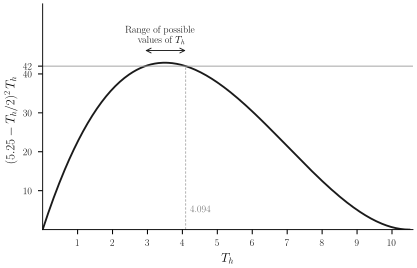 cates that the maximum value of \(T_{h}\), for winch the ordinate is greater than 42, is
\[ T_{h}=4.095 \quad\left(\text { or } T_{h}=409.5 \mathrm{~K}\right) \]
and furthermore that this value satisfies the equality, and therefore corresponds to a reversible process.
Another solution to this problem will be developed in Problem 4.6-7.
PROBLEMS
Problem 4.1-1
One mole of a monatomic ideal gas and one mole of an ideal van der Waals fluid (Section 3.5) with \(c=3 / 2\) are contained separately in vessels of fixed volumes \(v_{1}\) and \(v_{2}\). The temperature of the ideal gas is \(T_{1}\) and that of the van der Waals fluid is \(T_{2}\). It is desired to bring the ideal gas to temperature \(T_{2}\), maintaining the total energy constant. What is the final temperature of the van der Waals fluid? What restrictions apply among the parameters ( \(T_{1}, T_{2}, a, b, v_{1}, v_{2}\) ) if it is to be possible to design an engine to accomplish this temperature inversion (assuming, as always, that no external system is to be altered in the process)?
Problem 4.1-2
A rubber band (Section 3.7) is initially at temperature \(T_{B}\) and length \(L_{B}\).One mole of a monatomic ideal gas is initially at temperature \(T_{G}\) and volume \(V_{G}\).The ideal gas, maintained at constant volume \(V_{G}\), is to be heated to a final temperature \(T_{G}^{\prime}\). The energy required is to be supplied entirely by the rubber band. Need the length of the rubber band be changed, and, if so, by what amount?
Answer:
\[ \text { If } l \equiv L_{B}-L_{0}, \]
\[ l^{2}-\left(l^{\prime}\right)^{2} \geq 2 b^{-1} c L_{0}\left(L_{1}-L_{0}\right) \ln \left(1-\frac{3 R}{2 R L_{0}} \frac{T_{G}^{\prime}-T_{G}}{T_{B}}\right)+3 R b^{-1}\left(L_{1}-L_{0}\right) \ln \left(T_{G}^{1} / T_{G}\right) \]
Problem 4.1-3
Suppose the two systems in Example 1 were to have heat capacities of the form \(C(T)=D T^{n}\), with \(n>0\) :
Show that for such systems \(U=U_{0}+D T^{n+1} /(n+1)\) and \(S=S_{0}+D T^{n} / n\). What is the fundamental equation of such a system?
If the initial temperature of the two systems were \(T_{10}\) and \(T_{20}\) what would be the maximum delivered work (leaving the two systems at a common temperature)?
Answer:
- for \(n=2\) :
\[ W=\frac{D}{3}\left[T_{10}^{3}+T_{20}^{3}-\frac{1}{\sqrt{2}}\left(T_{10}^{2}+T_{20}^{2}\right)^{\frac{3}{2}}\right] \]
4-2 QUASI-STATIC AND REVERSIBLE PROCESSES
The central principle of entropy maximization spawns various theorems of more specific content when specialized to particular classes of processes. We shall turn our attention to such theorems after a preliminary refinement of the descriptions of states and of processes.
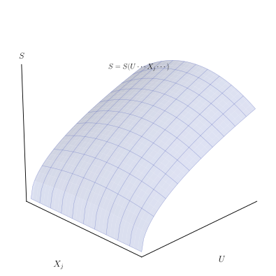
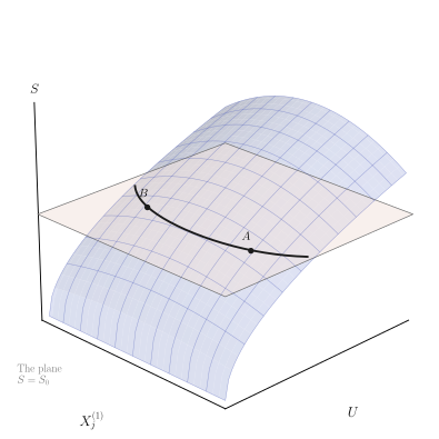
To describe and characterize thermodynamic states, and then to describe possible processes, it is useful to define a thermodynamic configuration space. The thermodynamic configuration space of a simple system is an abstract space spanned by coordinate axes that correspond to the entropy \(S\) and to the extensive parameters \(U, V, N_{1}, \ldots, N_{r}\) of the system. The fundamental equation of the system \(S=S\left(U, V, N_{1}, \ldots, N_{r}\right)\) defines a surface in the thermodynamic configuration space, as indicated schematically in Fig. 4.1. It should be noted that the surface of Fig. 4.1 conforms to the requirements that \((\partial S / \partial U) \ldots, x_{j}, \ldots(\equiv 1 / T)\) be positive, and that \(U\) be a single valued function of \(S, \ldots, x_{j}, \ldots\).
By definition, each point in the configuration space represents an equilibrium state. Representation of a nonequilibrium state would require a space of immensely greater dimension.
The fundamental equation of a composite system can be represented by a surface in a thermodynamic configuration space with coordinate axes
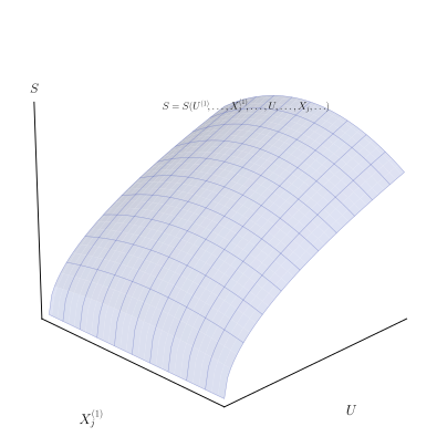
corresponding to the extensive parameters of all of the subsystems. For a composite system of two simple subsystems the coordinate axes can be associated with the total entropy \(S\) and the extensive parameters of the two subsystems. A more convenient choice is the total entropy \(S\), the extensive parameters of the first subsystem ( \(U^{(1)}, V^{(1)}, N_{1}^{(1)}, N_{2}^{(1)}, \ldots\) ), and the extensive parameters of the composite system ( \(U, V, N_{1}, N_{2}, \ldots\) ). An appropriate section of the thermodynamic configuration space of a composite system is sketched in Fig. 4.2.
Consider an arbitrary curve drawn on the hypersurface of Fig. 4.3, from an initial state to a terminal state. Such a curve is known as a quasi-static locus or a quasi-static process. A quasi-static process is thus defined in terms of a dense succession of equilibrium states. It is to be stressed that a quasi-static process therefore is an idealized concept, quite distinct from a real physical process, for a real process always involves nonequilibrium intermediate states having no representation in the thermodynamic configuration space. Furthermore, a quasi-static process, in contrast to a real process, does not involve considerations of rates, velocities, or time. The quasi-static process simply is an ordered succession of equilibrium states, whereas a real process is a temporal succession of equilibrium and nonequilibrium states.
Although no real process is identical to a quasi-static process, it is possible to contrive real processes that have a close relationship to quasi-static processes. In particular, it is possible to 1 a system through a succession of states that coincides at any desired n. aber of points with
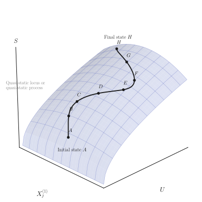
a given quasi-static locus. Thus consider a system originally in the state \(A\) of Fig. 4.3, and consider the quasi-static locus passing through the points \(A, B, C, \ldots, H\). We remove a constraint which permits the system to proceed from \(A\) to \(B\) but not to points further along the locus. The system “disappears” from the point \(A\) and subsequently appears at \(B\), having passed en route through nonrepresentable nonequilibrium states. If the constraint is further relaxed, making the state \(C\) accessible, the system disappears from \(B\) and subsequently reappears at \(C\). Repetition of the operation leads the system to states \(D, E, \ldots, H\). By such a succession of real processes we construct a process that is an approximation to the abstract quasi-static process shown in the figure. By spacing the points \(A, B, C, \ldots\) arbitrarily closely along the quasi-static locus we approximate the quasi-static locus arbitrarily closely.
The identification of \(-P d V\) as the mechanical work and of \(T d S\) as the heat transfer is valid only for quasi-static processes.
Consider a closed system that is to be led along the sequence of states \(A, B, C, \ldots, H\) approximating a quasi-static locus. The system is induced to go from \(A\) to \(B\) by the removal of some internal constraint. The closed system proceeds to \(B\) if (and only if) the state \(B\) has maximum entropy among all newly accessible states. In particular the state \(B\) must have higher entropy than the state \(A\). Accordingly, the physical process joining states \(A\) and \(B\) in a closed system has unique directionality. It proceeds from the state \(A\), of lower tropy, to the state \(B\), of higher entropy, but not inversely. Such processes are irreversible.
A quasi-static locus can be approxi ’ed by a real process in a closed system only if the entropy is monotonically nondecreasing along the quasistatic locus.
The limiting case of a quasi-static process in which the increase in the entropy becomes vanishingly small is called a reversible process (Fig. 4.4). For such a process the final entropy is equal to the initial entropy, and the process can be traversed in either direction.
PROBLEMS
Problem 4.2-1
Does every reversible process coincide with a quasi-static locus? Does every quasi-static locus coincide with a reversible process? For any real process starting in a state \(A\) and terminating in a state \(H\), does there exist some quasi-static locus with the same two terminal states \(A\) and \(H\) ? Does there exist some reversible process with the same two terminal states?
Problem 4.2-2
Consider a monatomic ideal gas in a cylinder fitted with a piston. The walls of the cylinder and the piston are adiabatic. The system is initially in equilibrium, but the external pressure is slowly decreased. The energy change of the gas in the resultant expansion \(d V\) is \(d U=-P d V\). Show, from equation 3.34, that \(d S=0\), so that the quasi-static adiabatic expansion is isentropic and reversible.
Problem 4.2-3
A monatomic ideal gas is permitted to expand by a free expansion from \(V\) to \(V+d V\) (recall Problem 3.4-8). Show that
\[ d S=\frac{N R}{V} d V \]
In a series of such infinitesimal free expansions, leading from \(V_{i}\) to \(V_{f}\), show that
\[ \Delta S=N R \ln \left(\frac{V_{f}}{V_{i}}\right) \]
Whether this atypical (and infamous) “continuous free expansion” process should be considered as quasi-static is a delicate point. On the positive side is the observation that the terminal states of the infinitesimal expansions can be spaced as closely as one wishes along the locus. On the negative side is the realization that the system necessarily passes through nonequilibrium states during each expansion; the irreversibility of the microexpansions is essential and irreducible. The fact that \(d S>0\) whereas \(d Q=0\) is inconsistent with the presumptive applicability of the relation \(d Q=T d S\) to all quasi-static processes. We define (by somewhat circular logic!) the continuous free expansion process as being “essentially irreversible” and non-quasi-static.
Problem 4.2-4
In the temperature range of interest a system obeys the equations
\[ T=A v^{2} / s \quad P=-2 A v \ln \left(s / s_{0}\right) \]
where \(A\) is a positive constant. The system undergoes a free expansion from \(v_{0}\) to \(v_{f}\) (with \(v_{f}>v_{0}\) ). Find the final temperature \(T_{f}\) in terms of the initial temperature \(T_{0}, v_{0}\), and \(v_{f}\). Find the increase in molar entropy.
4-3 RELAXATION TIMES AND IRREVERSIBILITY
Consider a system that is to be led along the quasi-static locus of Fig. 4.3. The constraints are to be removed step by step, the system being permitted at each step to come to a new equilibrium state lying on the locus. After each slight relaxation of a constraint we must wait until the system fully achieves equilibrium, then we proceed with the next slight relaxation of the constraint and we wait again, and so forth. Although this is the theoretically prescribed procedure, the practical realization of the process seldom follows this prescription. In practice the constraints usually are relaxed continuously, at some “sufficiently slow” rate.
The rate at which constraints can be relaxed as a system approximates a quasi-static locus is characterized by the relaxation time \(\tau\) of the system. For a given system, with a given relaxation time \(\tau\), processes that occur in times short compared to \(\tau\) are not quasi-static, whereas processes that occur in times long compared to \(\tau\) can be approximately quasi-static.
The physical considerations that determine the relaxation time can be illustrated by the adiabatic expansion of a gas (recall Problem 4.2-2). If the piston is permitted to move outward only extremely slowly the process is quasi-static (and reversible). If, however, the external pressure is decreased rapidly the resulting rapid motion of the piston is accompanied by turbulence and inhomogeneous flow within the cylinder (and by an entropy increase that “drives” these processes). The process is then neither quasi-static nor reversible. To estimate the relaxation time we first recognize that a slight outward motion of the piston reduces the density of the gas immediately adjacent to the piston. If the expansion is to be reversible this local “rarefaction” in the gas must be homogenized by hydrodynamic flow processes before the piston again moves appreciably. The rarefaction itself propagates through the gas with the velocity of sound, reflects from the walls of the cylinder, and gradually dissipates. The mechanism of dissipation involves both diffusive reflection from the walls and viscous damping within the gas. The simplest case would perhaps be that in which the cylinder walls are so rough that a single reflection would effectively dissipate the rarefaction pulse-admittedly not the common situation, but sufficient for our purely illustrative purposes. Then the relaxation time would be on the order of the time required for the rarefaction to propagate across the system, or \(\tau \simeq V^{\frac{1}{3}} / c\), where the cube root of the volume is taken as a measure of the “length” of the system and \(c\) is the velocity of sound in the gas. If the adiabatic expansion of the gas in the cylinder is performed in times much longer than this relaxation time the expansion occurs reversibly and isentropically. If the expansion is performed in times comparable to or shorter than the relaxation time there is an irreversible increase in entropy within the system and the expansion, though adiabatic, is not isentropic.
PROBLEMS
Problem 4.3-1
A cylinder of length \(L\) and cross-sectional area \(A\) is divided into two equal-volume chambers by a piston, held at the midpoint of the cylinder by a setscrew. One chamber of the cylinder contains \(N\) moles of a monatomic ideal gas at temperature \(T_{0}\). This same chamber contains a spring connected to the piston and to the end-wall of the cylinder; the unstretched length of the spring is \(L / 2\), so that it exerts no force on the piston when the piston is at its initial midpoint position. The force constant of the spring is \(K_{\text {spring }}\). The other chamber of the cylinder is evacuated. The setscrew is suddenly removed. Find the volume and temperature of the gas when equilibrium is achieved. Assume the walls and the piston to be adiabatic and the heat capacities of the spring, piston, and walls to be negligible.
Discuss the nature of the processes that lead to the final equilibrium state. If there were gas in each chamber of the cylinder the probler stated would be stated would be indeterminate! Why?
4-4 HEAT FLOW: COUPLED SYSTEMS AND REVERSAL OF PROCESSES
Perhaps the most characteristic of all thermodynamic processes is the quasi-static transfer of heat between two systems, and it is instructive to examine this process with some care.
In the simplest case we consider the transfer of heat \(d Q\) from one system at temperature \(T\) to another at the same temperature. Such a process is reversible, the increase in entropy of the recipient subsystem \(d Q / T\) being exactly counterbalanced by the decrease in entropy \(-d Q / T\) of the donor subsystem.
In contrast, suppose that the two subsystems have different initial temperatures \(T_{10}\) and \(T_{20}\), with \(T_{10}<T_{20}\). Further, let the heat capacities (at constant volume) be \(C_{1}(T)\) and \(C_{2}(T)\). Then if a quantity of heat \(d Q_{1}\) is quasi-statically inserted into system 1 (at constant volume) the entropy increase is
\[ d S_{1}=\frac{d Q_{1}}{T_{1}}=C_{1}\left(T_{1}\right) \frac{d T_{1}}{T_{1}} \]
and similarly for subsystem 2 . If such infinitesimal transfers of heat from the hotter to the colder body continue until the two temperatures become equal, then energy conservation requires
\[ \Delta U=\int_{T_{10}}^{T_{f}} C_{1}\left(T_{1}\right) d T_{1}+\int_{T_{20}}^{T_{f}} C_{2}\left(T_{2}\right) d T_{2}=0 \]
which determines \(T_{f}\). The resultant change in entropy is
\[ \Delta S=\int_{T_{10}}^{T_{f}} \frac{C_{1}\left(T_{1}\right)}{T_{1}} d T_{1}+\int_{T_{20}}^{T_{f}} \frac{C_{2}\left(T_{2}\right)}{T_{2}} d T_{2} \]
In the particular case in which \(C_{1}\) and \(C_{2}\) are independent of \(T\) the energy conservation condition gives
\[ T_{f}=\frac{C_{1} T_{10}+C_{2} T_{20}}{C_{1}+C_{2}} \]
and the entropy increase is
\[ \Delta S=C_{1} \ln \left(\frac{T_{f}}{T_{10}}\right)+C_{2} \ln \left(\frac{T_{f}}{T_{20}}\right) \]
It is left to Problem 4.4-3 ’emonstrate that this expression for \(\Delta S\) is intrinsically positive.
Several aspects of the heat transfer process deserve reflection. First, we note that the process, though quasi-static, is irreversible; it is represented in thermodynamic configuration space by a quasi-static locus of monotonically increasing \(S\).
Second, the process can be associated with the spontaneous flow of heat from a hot to a cold system providing \((a)\) that the intermediate wall through which the heat flow occurs is thin enough that its mass (and hence its contribution to the thermodynamic properties of the system) is negligible, and \((b)\) that the rate of heat flow is sufficiently slow (i.e., the thermal resistivity of the wall is sufficiently high) that the temperature remains spatially homogeneous within each subsystem.
Third, we note that the entropy of one of the subsystems is decreased, whereas that of the other subsystem is increased. It is possible to decrease the entropy of any particular system, providing that this decrease is linked to an even greater entropy increase in some other system. In this sense an irreversible process within a given system can be “reversed”-with the hidden cost paid elsewhere.
PROBLEMS
Problem 4.4-1
Each of two bodies has a heat capacity given, in the temperature range of interest, by
\[ C=A+B T \]
where \(A=8 \mathrm{~J} / \mathrm{K}\) and \(B=2 \times 10^{-2} \mathrm{~J} / \mathrm{K}^{2}\). If the two bodies are initially at temperatures \(T_{10}=400 \mathrm{~K}\) and \(T_{20}=200 \mathrm{~K}\), and if they are brought into thermal contact, what is the final temperature and what is the change in entropy?
Problem 4.4-2
Consider again the system of Problem 4.4-1. Let a third body be available, with heat capacity
\[ C_{3}=B T \]
and with an initial temperature of \(T_{30}\). Bodies 1 and 2 are separated, and body 3 is put into thermal contact with body 2 . What must the initial temperature \(T_{30}\) be in order thereby to restore body 2 to its initial state? By how much is the entropy of body 2 decreased in this second process?
Problem 4.4-3
Prove that the entropy change in a heat flow process, as given in equation 4.5, is intrinsically positive.
Problem 4.4-4
Show that if two bodies have equal heat capacities, each of which is constant (independent of temperature), the equilibrium temperature achieved by direct thermal contact is the arithmetic average of the initial temperatures.
Problem 4.4-5
Over a limited temperature range the heat capacity at constant volume of a particular type of system is inversely proportional to the temperature.
What is the temperature dependence of the energy, at constant volume, for this type of system?
If two such systems, at initial temperatures \(T_{10}\) and \(T_{20}\), are put into thermal contact what is the equilibrium temperature of the pair?
Problem 4.4-6
A series of \(N+1\) large vats of water have temperatures \(T_{0}, T_{1}, T_{2}, \ldots, T_{N}\) (with \(T_{n}>T_{n-1}\) ). A small body with heat capacity \(C\) (and with a constant volume, independent of temperature) is initially in thermal equilibrium with the vat of temperature \(T_{0}\). The body is removed from this vat and immersed in the vat of temperature \(T_{1}\). The process is repeated until, after \(N\) steps, the body is in equilibrium with the vat of temperature \(T_{N}\). The sequence is then reversed, until the body is once again in the initial vat, at temperature \(T_{0}\). Assuming the ratio of temperatures of successive vats to be a constant, or
\[ T_{n} / T_{n-1}=\left(T_{N} / T_{0}\right)^{1 / N} \]
and neglecting the (small) change in temperature of any vat, calculate the change in total entropy as
- the body is successively taken “up the sequence” (from \(T_{0}\) to \(T_{N}\) ), and \(b\) ) the body is brought back “down the sequence” (from \(T_{N}\) to \(T_{0}\) ). What is the total change in entropy in the sum of the two sequences above? Calculate the leading nontrivial limit of these results as \(N \rightarrow \infty\), keeping \(T_{0}\) and \(T_{N}\) constant. Note that for large \(N\)
\[ N\left(x^{1 / N}-1\right) \simeq \ln x+(\ln x)^{2} / 2 N+\cdots \]
4-5 THE MAXIMUM WORK THEOREM
The propensity of physical systems to increase their entropy can be channeled to deliver useful work. All such applications are governed by the maximum work theorem.
Consider a system that is to be taken from a specified initial state to a specified final state. Also available are two auxiliary systems, into one of which work can be transferred, and into the other of which heat can be transferred. Then the maximum work theorem states that for all processes leading from the specified initial state to the specified final state of the primary system, the delivery of work is maximum (and the delivery of heat is minimum) for a reversible process. Furthermore the delivery of work (and of heat) is identical for every reversible process.
The repository system into which work is delivered is called a “reversible work source.” Reversible work sources are defined as systems enclosed by adiabatic impermeable walls and characterized by relaxation times sufficiently short that all processes within them are essentially quasi-static. From the thermodynamic point of view the “conservative” (nonfrictional) systems considered in the theory of mechanics are reversible work sources.
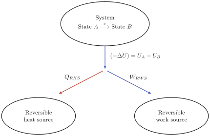
The repository system into which heat is delivered is called a “reversible heat source” \({ }^{1}\). Reversible heat sources are defined as systems enclosed by rigid impermeable walls and characterized by relaxation times sufficiently short that all processes of interest within them are essentially quasi-static. If the temperature of the reversible heat source is \(T\) the transfer of heat \(d Q\) to the reversible heat source increases its entropy according to the quasistatic relationship \(d Q=T d S\). The external interactions of a reversible heat source accordingly are fully described by its heat capacity \(C(T)\) (the definition of the reversible heat source implies that this heat capacity is at constant volume, but we shall not so indicate by an explicit subscript). The energy change of the reversible heat source is \(d U=d Q=C(T) d T\) and the entropy change is \(d S=[C(T) / T] d T\). The various transfers envisaged in the maximum work theorem are indicated schematically in Fig. 4.5.
The proof of the maximum work theorem is almost immediate. Consider two processes. Each leads to the same energy change \(\Delta U\) and the same entropy change \(\Delta S\) within the primary subsystem, for these are determined by the specified initial and final states. The two processes differ only in the apportionment of the energy difference ( \(-\Delta U\) ) between the reversible work source and the reversible heat source ( \(-\Delta U=W_{\mathrm{RWS}}\) \(+Q_{\mathrm{RHS}}\) ). But the process that delivers the maximum possible work to the reversible work source correspondingly delivers the least possible heat to the reversible heat source, and therefore leads to the least possible entropy increase of the reversible heat source (and thence of the entire system).
[^8]The absolute minimum of \(\Delta S_{\text {total }}\), for all possible processes, is attained by any reversible process (for all of which \(\Delta S_{\text {total }}=0\) ).
To recapitulate, energy conservation requires \(\Delta U+W_{\mathrm{RWS}}+Q_{\mathrm{RHS}}=0\). With \(\Delta U\) fixed, to maximize \(W_{\mathrm{RWS}}\) is to minimize \(Q_{\mathrm{RHS}}\). This is achieved by minimizing \(S_{\text {RHS }}^{\text {final }}\) (since \(S_{\text {RHS }}\) increases monotonically with positive heat input \(Q_{\mathrm{RHS}}\) ). The minimum \(S_{\mathrm{RHS}}^{\text {final }}\) therefore is achieved by minimum \(\Delta S_{\text {total }}\), or by \(\Delta S_{\text {total }}=0\).
The foregoing “descriptive” proof can be cast into more formal language, and this is particularly revealing in the case in which the initial and final states of the subsystem are so close that all differences can be expressed as differentials. Then energy conservation requires
\[ d U+d Q_{\mathrm{RHS}}+d W_{\mathrm{RWS}}=0 \]
whereas the entropy maximum principle requires
\[ d S_{\mathrm{tot}}=d S+\frac{d Q_{\mathrm{RHS}}}{T_{\mathrm{RHS}}} \geq 0 \]
It follows that
\[ d W_{\mathrm{RWS}} \leq T_{\mathrm{RHS}} d S-d U \]
The quantities on the right-hand side are all specified. In particular \(d S\) and \(d U\) are the entropy and energy differences of the primary subsystem in the specified final and initial states. The maximum work transfer \(d W_{\text {RWS }}\) corresponds to the equality sign in equation 4.8, and therefore in equation \(4.7\left(d S_{\text {tot }}=0\right)\).
It is useful to calculate the maximum delivered work which, from equation 4.8 and from the identity \(d U=d Q+d W\), becomes
\[ \begin{aligned} d W_{\mathrm{RWS}} \text { (maximum) } & =\left(\frac{T_{\mathrm{RHS}}}{T}\right) d Q-d U \\ & =\left[1-\left(T_{\mathrm{RHS}} / T\right)\right](-d Q)+(-d W) \end{aligned} \]
That is, in an initesimal process, the maximum work that can be delivered to the reversible work source is the sum of:
- the work ( \(-d W\) ) directly extracted from the subsystem,
- a fraction ( \(1-T_{\mathrm{RHS}} / T\) ) of the heat ( \(-d Q\) ) directly extracted from the subsystem.
The fraction ( \(1-T_{\text {RHS }} / T\) ) of the extracted heat that can be “converted” to work in an infinitesimal process is called the thermodynamic engine efficiency, and we shall return to a discussion of that quantity in Section 4.5. However, it generally is preferable to solve maximum work problems in terms of an overall accounting of energy and entropy changes (rather than to integrate over the thermodynamic engine efficiency).
Returning to the total (noninfinitesimal) process, the energy conservation condition becomes
\[ \Delta U_{\text {subsystem }}+Q_{\mathrm{RHS}}+W_{\mathrm{RWS}}=0 \]
whereas the reversibility condition is
\[ \Delta S_{\text {total }}=\Delta S_{\text {subsystem }}+\int d Q_{\mathrm{RHS}} / T_{\mathrm{RHS}}=0 \]
In order to evaluate the latter integral it is necessary to know the heat capacity \(C_{\text {RHS }}(T)=d Q_{\text {RHS }} / d T_{\text {RHS }}\) of the reversible heat source. Given \(C_{\text {RHS }}(T)\) the integral can be evaluated, and one can then also infer the net heat transfer \(Q_{\text {RHS }}\). Equation 4.10 in turn evaluates \(W_{\text {RWS }}\). Equations 4.10 and 4.11, evaluated as described, provide the solution of all problems based on the maximum work theorem.
The problem is further simplified if the reversible heat source is a thermal reservoir. A thermal reservoir is defined as a reversible heat source that is so large that any heat transfer of interest does not alter the temperature of the thermal reservoir. Equivalently, a thermal reservoir is a reversible heat source characterized by a fixed and definite temperature. For such a system equation 4.11 reduces simply to
\[ \Delta S_{\text {total }}=\Delta S_{\text {subsystem }}+\frac{Q_{\text {res }}}{T_{\text {res }}}=0 \]
and \(Q_{\text {res }}\left(=Q_{\text {RHS }}\right)\) can be eliminated between equations 4.10 and 4.12, giving
\[ W_{\mathrm{RWS}}=T_{\mathrm{res}} \Delta S_{\text {subsystem }}-\Delta U_{\text {subsystem }} \]
Finally, it should be recognized that the specified final state of the subsystem may have a larger energy than the initial state. In that case the theorem remains formally true but the “delivered work” may be negative. This work which must be supplied to the subsystem will then be least (the delivered work remains algebraically maximum) for a reversible process.
Example 1
One mole of an ideal van der Waals fluid is to be taken by an unspecified process from the state \(T_{0}, v_{0}\) to the state \(T_{f}, v_{f}\). A second system is constrained to have a fixed volume and its initial temperature is \(T_{20}\); its heat capacity is linear in the temperature
\[ C_{2}(T)=D T \quad(D=\text { constant }) \]
What is the maximum work that can be delivered to a reversible work source? Solution The solution parallels those of the problems in Section 4.1 despite the slightly different formulations. The second system is a reversible heat source; for it the dependence of energy on temperature is
\[ U_{2}(T)=\int C_{2}(T) d T=\frac{1}{2} D T^{2}+\text { constant } \]
and the dependence of entropy on temperature is
\[ S_{2}(T)=\int \frac{C_{2}(T)}{T} d T=D T+\text { constant } \]
For the primary fluid system the dependence of energy and entropy on \(T\) and \(v\) is given in equations 3.49 and 3.51 from which we find
\[ \begin{aligned} & \Delta U_{1}=c R\left(T_{f}-T_{0}\right)-\frac{a}{v_{f}}+\frac{a}{v_{0}} \\ & \Delta S_{1}=R \ln \left(\frac{v_{f}-b}{v_{0}-b}\right)+c R \ln \frac{T_{f}}{T_{0}} \end{aligned} \]
The second system (the reversible heat source) changes temperature from \(T_{20}\) to some as yet unknown temperature \(T_{2 f}\), so that
\[ \Delta U_{2}=\frac{1}{2} D\left(T_{2 f}^{2}-T_{20}^{2}\right) \]
and
\[ \Delta S_{2}=D\left(T_{2 f}-T_{20}\right) \]
The value of \(T_{2 f}\) is determined by the reversibility condition
\[ \Delta S_{1}+\Delta S_{2}=R \ln \left(\frac{v_{f}-b}{v_{0}-b}\right)+c R \ln \frac{T_{f}}{T_{0}}+D\left(T_{2 f}-T_{20}\right)=0 \]
or
\[ T_{2 f}=T_{20}-R D^{-1} \ln \left(\frac{v_{f}-b}{v_{0}-b}\right)-c R D^{-1} \ln \frac{T_{f}}{T_{0}} \]
The conservation of energy then determines the work \(W_{3}\) delivered to the reversible work source
\[ W_{3}+\Delta U_{2}+\Delta U_{1}=0 \]
whence
\[ W_{3}=-\left[\frac{1}{2} D\left(T_{2 f}^{2}-T_{20}^{2}\right)\right]-\left[c R\left(T_{f}-T_{0}\right)-\frac{a}{v_{f}}+\frac{a}{v_{0}}\right] \]
where we recall that \(T_{f}\) is given, whereas \(T_{2 f}\) has been found.
An equivalent problem, but with a somewhat simpler system (a monatomic ideal gas and a thermal reservoir) is formulated in Problem 4.5-1. In each of these problems we do not commit ourselves to any specific process by which the result might be realized, but such a specific process is developed in Problem 4.5-2 (which, with 4.5-1, is strongly recommended to the reader).
Example 2 Isotope Separation
In the separation of \(\mathrm{U}^{235}\) and \(\mathrm{U}^{238}\) to produce enriched fuels for atomic power plants the naturally occurring uranium is reacted with fluorine to form uranium hexafluoride \(\left(\mathrm{UF}_{6}\right)\). The uranium hexafluoride is a gas at room temperature and atmospheric pressure. The naturally occurring mole fraction of \(\mathbf{U}^{235}\) is 0.0072, or \(0.72 \%\). It is desired to process 10 moles of natural \(\mathrm{UF}_{6}\) to produce 1 mole of \(2 \%\) enriched material, leaving 9 moles of partially depleted material. The \(\mathrm{UF}_{6}\) gas can be represented approximately as a polyatomic, multicomponent simple ideal gas with \(c=7 / 2\) (equation 3.40). Assuming the separation process to be carried out at a temperature of 300 K and a pressure of 1 atm , and assuming the ambient atmosphere (at 300 K) to act as a thermal reservoir, what is the minimum amount of work required to carry out the enrichment process? Where does this work (energy) ultimately reside?
Solution
The problem is an example of the maximum work theorem in which the minimum work required corresponds to the maximum work “delivered.” The initial state of the system is 10 moles of natural \(\mathrm{UF}_{6}\) at \(T=300 \mathrm{~K}\) and \(P=1 \mathrm{~atm}\). The final state of the system is 1 mole of enriched gas and 9 moles of depleted gas at the same temperature and pressure. The cold reservoir is also at the same temperature.
We find the changes of entropy and of energy of the system. From the fundamental equation (3.40) we find the equations of state to be the familiar forms
\[ U=7 / 2 \mathrm{NRT} \quad P V=\mathrm{NRT} \]
These enable us to write the entropy as a function of \(T\) and \(P\).
\[ S=\sum_{j=1}^{2} N_{j} s_{0 j}+\left(\frac{7}{2}\right) N R \ln \left(\frac{T}{T_{0}}\right)-N R \ln \left(\frac{P}{P_{0}}\right)-N R \sum_{j=1}^{2} x_{j} \ln x_{j} \]
This last term-the “entropy of mixing” as defined following equation 3.40-is the significant term in the isotope separation process.
We first calculate the mole fraction of \(\mathrm{U}^{235} \mathrm{~F}_{6}\) in the 9 moles of depleted material; this is found to be \(0.578 \%\). Accordingly the change in entropy is
\[ \begin{aligned} \Delta S= & -R[0.02 \ln 0.02+0.98 \ln 0.98]-9 R[0.00578 \ln 0.00578 \\ & +0.994 \ln 0.994]+10 R[0.0072 \ln 0.0072+0.9928 \ln 0.9928] \\ = & -0.0081 R=-0.067 \mathrm{~J} / \mathrm{K} \end{aligned} \]
The gas ejects heat.
There is no change in the energy of the gas, and all the energy supplied as work is transferred to the ambient atmosphere as heat. That work, or heat, is
\[ -W_{\mathrm{RWS}}=Q_{\mathrm{res}}=-T \Delta S=300 \times 0.067=20 \mathrm{~J} \]
If there existed a semipermeable membrane, permeable to \(\mathrm{U}^{235} \mathrm{~F}_{6}\) but not to \(\mathrm{U}^{238} \mathrm{~F}_{6}\), the separation could be accomplished simply. Unfortunately no such membrane exists. The methods employed in practice are all dynamic (non-quasistatic) processes that exploit the small mass difference of the two isotopes-in ultracentrifuges, in mass spectrometers, or in gaseous diffusion.
PROBLEMS
Problem 4.5-1
One mole of a monatomic ideal gas is contained in a cylinder of volume \(10^{-3} \mathrm{~m}^{3}\) at a temperature of 400 K. The gas is to be brought to a final state of volume \(2 \times 10^{-3} \mathrm{~m}^{3}\) and temperature 400 K. A thermal reservoir of temperature 300 K is available, as is a reversible work source. What is the maximum work that can be delivered to the reversible work source?
Answer:
\[ W_{\mathrm{RWS}}=300 R \ln 2 \]
Problem 4.5-2
Consider the following process for the system of Problem 4.5-1. The ideal gas is first expanded adiabatically (and isentropically) until its temperature falls to 300 K; the gas does work on the reversible work source in this expansion. The gas is then expanded while in thermal contact with the thermal reservoir. And finally the gas is compressed adiabatically until its volume and temperature reach the specified values ( \(2 \times 10^{-3} \mathrm{~m}^{3}\) and 400 K ).
Draw the three steps of this process on a \(T-V\) diagram, giving the equation of each curve and labelling the numerical coordinates of the vertices.
To what volume must the gas be expanded in the second step so that the third (adiabatic) compression leads to the desired final state?
Calculate the work and heat transfers in each step of the process and show that the overall results are identical to those obtained by the general approach of Example 1.
Problem 4.5-3
Describe how the gas of the preceding two problems could be brought to the desired final state by a free expansion. What are the work and heat transfers in this case? Are these results consistent with the maximum work theorem?
Problem 4.5-4
The gaseous system of Problem 4.5-1 is to be restored to its initial state. Both states have temperature 400 K, and the energies of the two states are equal \((U=600 R)\). Need any work be supplied, and if so, what is the minimum supplied work? Note that the thermal reservoir of temperature 300 K remains accessible.
Problem 4.5-5
If the thermal reservoir of Problem 4.5-1 were to be replaced by a reversible heat source having a heat capacity of the form
\[ C(T)=\left(2+\frac{T}{150}\right) R \]
and an initial temperature of \(T_{\mathrm{RHS}, 0}=300 \mathrm{~K}\), again calculate the maximum delivered work.
Before doing the calculation, would you expect the delivered work to be greater, equal to, or smaller than that calculated in Prob. 4.5-1? Why?
Problem 4.5-6
A system can be taken from state \(A\) to state \(B\) (where \(S_{B}=S_{A}\) ) either ( \(a\) ) directly along the adiabat \(S=\) constant, or ( \(b\) ) along the isochore \(A C\) and the isobar \(C B\). The difference in the work done by the system is the area enclosed between the two paths in a \(P-V\) diagram. Does this contravene the statement that the work delivered to a reversible work source is the same for every reversible process? Explain!
Problem 4.5-7
Consider the maximum work theorem in the case in which the specified final state of the subsystem has lower energy than the initial state. Then the essential logic of the theorem can be summarized as follows: “Extraction of heat from the subsystem decreases its entropy. Consequently a portion of the extracted heat must be sacrificed to a reversible heat source to effect a net increase in entropy; otherwise the process will not proceed. The remainder of the extracted heat is available as work.”
Similarly summarize the essential logic of the theorem in the case in which the final state of the subsystem has larger energy and larger entropy than the initial state.
Problem 4.5-8
If \(S_{B}<S_{A}\) and \(U_{B}>U_{A}\) does this imply that the delivered work is negative? Prove your assertion assuming the reversible heat source to be a thermal reservoir.
Does postulate III, which states that \(S\) is a monotonically increasing function of \(U\), disbar the conditions assumed here? Explain.
Problem 4.5-9
Two identical bodies each have constant and equal heat capacities ( \(C_{1}=\) \(C_{2}=C\), a constant). In addition a reversible work source is available. The initial temperatures of the two bodies are \(T_{10}\) and \(T_{20}\). What is the maximum work that can be delivered to the reversible work source, leaving the two bodies in thermal equilibrium? What is the corresponding equilibrium temperature? Is this the minimum attainable equilibrium temperature, and if so, why? What is the maximum attainable equilibrium temperature?
For \(C=8 \mathrm{~J} / \mathrm{K}, T_{10}=100^{\circ} \mathrm{C}\) and \(T_{20}=0^{\circ} \mathrm{C}\) calculate the maximum delivered work and the possible range of final equilibrium temperature.
Answer:
\[ \begin{gathered} T_{f}^{\min }=46^{\circ} \mathrm{C} \quad T_{f}^{\max }=50^{\circ} \mathrm{C} \\ W^{\max }=C\left[\sqrt{T_{10}}-\sqrt{T_{20}}\right]^{2}=62.2 \mathrm{~J} \end{gathered} \]
Problem 4.5-10
Two identical bodies each have heat capacities (at constant volume) of
\[ C(T)=a / T \]
The initial temperatures are \(T_{10}\) and \(T_{20}\), with \(T_{20}>T_{10}\). The two bodies are to be brought to thermal equilibrium with each other (maintaining both volumes constant) while delivering as much work as possible to a reversible work source. What is the final equilibrium temperature and what is the maximum work delivered to the reversible work source?
Evaluate your answer for \(T_{20}=T_{10}\) and for \(T_{20}=2 T_{10}\). Answer:
\[ W=a \ln (9 / 8) \text { if } T_{20}=2 T_{10} \]
Problem 4.5-11
Two bodies have heat capacities (at constant volume) of
\[ \begin{aligned} & C_{1}=a T \\ & C_{2}=2 b T \end{aligned} \]
The initial temperatures are \(T_{10}\) and \(T_{20}\), with \(T_{20}>T_{10}\). The two bodies are to be brought to thermal equilibrium (maintaining both volumes constant) while delivering as much work as possible to a reversible work source. What is the final equilibrium temperature and what is the (maximum) work delivered to the reversible work source?
Problem 4.5-12
One mole of an ideal van der Waals fluid is contained in a cylinder fitted with a piston. The initial temperature of the gas is \(T_{t}\) and the initial volume is \(v_{i}\). A reversible heat source with a constant heat capacity \(C\) and with an initial temperature \(T_{0}\) is available. The gas is to be compressed to a volume of \(v_{f}\) and brought into thermal equilibrium with the reversible heat source. What is the maximum work that can be delivered to the reversible work source and what is the final temperature?
\[ T_{f}=\left[\left(\frac{v_{t}-b}{v_{f}-b}\right)^{R} T_{i}^{c R} T_{0}\right]^{\begin{array}{c} \text { Answer: } \\ 1 /(c R+C) \end{array}} \]
Problem 4.5-13
A system has a temperature-independent heat capacity \(C\). The system is initially at temperature \(T_{i}\) and a heat reservoir is available, at temperature \(T_{c}\) (with \(T_{c}<T_{i}\) ). Find the maximum work recoverable as the system is cooled to the temperature of the reservoir.
Problem 4.5-14
If the temperature of the atmosphere is 5°C on a winter day and if 1 kg of water at 90°C is available, how much work can be obtained as the water is cooled to the ambient temperature? Assume that the volume of the water is constant, and assume that the molar heat capacity at constant volume is \(75 \mathrm{~J} /\) mole K and is independent of temperature.
Answer:
\[ 45 \times 10^{3} \mathrm{~J} \]
Problem 4.5-15
A rigid cylinder contains an internal adiabatic piston separating it into two chambers, of volumes \(V_{10}\) and \(V_{20}\). The first chamber contains one mole of a monatomic ideal gas at temperature \(T_{10}\). The second chamber contains one mole of a simple diatomic ideal gas \((c=5 / 2)\) at temperature \(T_{20}\). In addition a thermal reservoir at temperature \(T_{c}\) is available. What is the maximum work that can be delivered to a reversible work source, and what are the corresponding volumes and temperatures of the two subsystems?
Problem 4.5-16
Each of three identical bodies has a temperature-independent heat capacity \(C\). The three bodies have initial temperatures \(T_{3}>T_{2}>T_{1}\). What is the maximum amount of work that can be extracted leaving the three bodies at a common final temperature?
Problem 4.5-17
Each of two bodies has a heat capacity given by
\[ C=A+2 B T \]
where \(A=8 \mathrm{~J} / \mathrm{K}\) and \(B=2 \times 10^{-2} \mathrm{~J} / \mathrm{K}^{2}\). If the bodies are initially at temperatures of 200 K and 400 K , and if a reversible work source is available, what is the minimum final common temperature to which the two bodies can be brought? If no work can be extracted from the reversible work source what is the maximum final common temperature to which the two bodies can be brought? What is the maximum amount of work that can be transferred to the reversible work source?
\[ \begin{array}{r} \text { Answer: } \\ T_{\min }=293 \mathrm{~K} \end{array} \]
Problem 4.5-18
A particular system has the equations of state
\[ T=A s / v^{1 / 2} \quad \text { and } \quad P=T^{2} / 4 A v^{1 / 2} \]
where \(A\) is a constant. One mole of this system is initially at a temperature \(T_{1}\) and volume \(V_{1}\). It is desired to cool the system to a temperature \(T_{2}\) while compressing it to volume \(V_{2}\left(T_{2}<T_{1} ; V_{2}<V_{1}\right)\). A second system is available. It is initially at a temperature \(T_{c}\left(T_{c}<T_{2}\right)\). Its volume is kept constant throughout, and its heat capacity is
\[ C_{V}=B T^{1 / 2} \quad(B=\text { constant }) \]
What is the minimum amount of work that must be supplied by an external agent to accomplish this goal?
Problem 4.5-19
A particular type of system obeys the equations
\[ T=\frac{u}{b} \quad \text { and } \quad P=a v T \]
where \(a\) and \(b\) are constants. Two such systems, each of 1 mole, are initially at temperatures \(T_{1}\) and \(T_{2}\) (with \(T_{2}>T_{1}\) ) and each has a volume \(v_{0}\). The systems are to be brought to a common temperature \(T_{f}\), with each at the same final volume \(v_{f}\). The process is to be such as to deliver maximum work to a reversible work source.
What is the final temperature \(T_{f}\) ?
How much work can be delivered? Express the result in terms of \(T_{1}, T_{2}, v_{0}, v_{f}\), and the constants \(a\) and \(b\).
Problem 4.5-20
Suppose that we have a system in some initial state (we may think of a tank of hot, compressed gas as an example) and we wish to use it as a source of work. Practical considerations require that the system be left finally at atmospheric temperature and pressure, in equilibrium with the ambient atmosphere. Show, first, that the system does work on the atmosphere, and that the work actually available for useful purposes is therefore less than that calculated by a straightforward application of the maximum work theorem. In engineering parlance this net available work is called the “availability”.
- Show that the availability is given by
\[ \text { Availability }=\left(U_{0}+P_{\mathrm{atm}} V_{0}-T_{\mathrm{atm}} S_{0}\right)-\left(U_{f}+P_{\mathrm{atm}} V_{f}-T_{\mathrm{atm}} S_{f}\right) \]
where the subscript \(f\) denotes the final state, in which the pressure is \(P_{\text {atm }}\) and the temperature is \(T_{\text {atm }}\).
- If the original system were to undergo an internal chemical reaction during the process considered, would that invalidate this formula for the availability?
Problem 4.5-21
An antarctic meteorological station suddenly loses all of its fuel. It has \(N\) moles of an inert “ideal van der Waals fluid” at a high temperature \(T_{h}\) and a high pressure \(P_{h}\). The (constant) temperature of the environment is \(T_{0}\) and the atmospheric pressure is \(P_{0}\). If operation of the station requires a continuous power \(\mathscr{P}\), what is the longest conceivable time, \(t_{\max }\), that the station can operate? Calculate \(t_{\text {max }}\) in terms of \(T_{h}, T_{0}, P_{h}, P_{0}, \mathscr{P}, N\) and the van der Waals constants \(a\), \(b\), and \(c\).
Note that this is a problem in availability, as defined and discussed in Problem \(4.5-20\). In giving the solution it is not required that the molar volume \(v_{h}\) be solved explicitly in terms of \(T_{h}\) and \(P_{h}\); it is sufficient simply to designate it as \(v_{h}\left(T_{h}, P_{h}\right)\) and similarly for \(v_{0}\left(T_{0}, P_{0}\right)\).
Problem 4.5-22
A “geothermal” power source is available to drive an oxygen production plant. The geothermal source is simply a well containing \(10^{3} \mathrm{~m}^{3}\) of water, initially at \(100^{\circ} \mathrm{C}\); nearby there is a huge (“infinite”) lake at \(5^{\circ} \mathrm{C}\). The oxygen is to be separated from air, the separation being carried out at 1 atm of pressure and at \(20^{\circ} \mathrm{C}\). Assume air to be \(\frac{1}{5}\) oxygen and \(\frac{4}{5}\) nitrogen (in mole fractions), and assume that it can be treated as a mixture of ideal gases. How many moles of \(\mathrm{O}_{2}\) can be produced in principle (i.e., assuming perfect thermodynamic efficiency) before exhausting the power source?
PROBLEMS
Problem 4.6-1
A temperature of 0.001 K is accessible in low temperature laboratories with moderate effort. If the price of energy purchased from the electric utility company is \(15 ¢ / \mathrm{kW} \mathrm{h}\) what would be the minimum cost of extraction of one watt-hour of heat from a system at 0.001 K? The “warm reservoir” is the ambient atmosphere at 300 K .
Answer: $45
Problem 4.6-2
A home is to be maintained at 70°F, and the external temperature is 50°F. One method of heating the home is to purchase work from the power company and to convert it directly into heat: This is the method used in common electric room heaters. Alternatively, the purchased work can be used to operate a heat pump. What is the ratio of the costs if the heat pump attains the ideal thermodynamic coefficient of performance?
Problem 4.6-3
A household refrigerator is maintained at a temperature of 35°F. Every time the door is opened, warm material is placed inside, introducing an average of 50 kcal, but making only a small change in the temperature of the refrigerator.
The door is opened 15 times a day, and the refrigerator operates at \(15 \%\) of the ideal coefficient of performance. The cost of work is \(15 ¢ / \mathrm{kW} \mathrm{h}\). What is the monthly bill for operating this refrigerator?
Problem 4.6-4
Heat is extracted from a bath of liquid helium at a temperature of 4.2 K. The high-temperature reservoir is a bath of liquid nitrogen at a temperature of 77.3 K. How many Joules of heat are introduced into the nitrogen bath for each Joule extracted from the helium bath?
Problem 4.6-5
Assume that a particular body has the equation of state \(U=N C T\) with \(N C=10 \mathrm{~J} / \mathrm{K}\) and assume that this equation of state is valid throughout the temperature range from 0.5 K to room temperature. How much work must be expended to cool this body from room temperature (300 K) to 0.5 K , using the ambient atmosphere as the hot reservoir?
Answer: 16.2 kJ.
Problem 4.6-6
One mole of a monatomic ideal gas is allowed to expand isothermally from an initial volume of 10 liters to a final volume of 15 liters, the temperature being maintained at 400 K . The work delivered is used to drive a thermodynamic refrigerator operating between reservoirs of temperatures 200 and 300 K. What is the maximum amount of heat withdrawn from the low-temperature reservoir?
Problem 4.6-7
Give a “constructive solution” of Example 2 of Section 4.1. Your solution may be based on the following procedure for achieving maximum temperature of the hot body. A thermodynamic engine is operated between the two cooler bodies, extracting work until the two cooler bodies reach a common temperature. This work is then used as the input to a heat pump, extracting heat from the cooler pair and heating the hot body. Show that this procedure leads to the same result as was obtained in the example.
Problem 4.6-8
Assume that 1 mole of an ideal van der Waals fluid is expanded isothermally, at temperature \(T_{h}\), from an initial volume \(V_{l}\) to a final volume \(V_{f}\). A thermal reservoir at temperature \(T_{c}\) is available. Apply equation 4.9 to a differential process and integrate to calculate the work delivered to a reversible work source. Corroborate by overall energy and entropy conservation.
Hint: Remember to add the direct work transfer \(P d V\) to obtain the total work delivered to the reversible work source (as in equation 4.9).
Problem 4.6-9
Two moles of a monatomic ideal gas are to be taken from an initial state \(\left(P_{i}, V_{i}\right)\) to a final state ( \(P_{f}=B^{2} P_{i}, V_{f}=V_{i} / B\) ), where \(B\) is a constant. A reversible work source and a thermal reservoir of temperature \(T_{c}\) are available. Find the maximum work that can be delivered to the reversible work source.
Given values of \(B, P_{i}\) and \(T_{c}\), for what values of \(V_{i}\) is the maximum delivered work positive?
Problem 4.6-10
Assume the process in Problem 4.6-9 to occur along the locus \(P=B / V^{2}\), where \(B=P_{i} V_{i}^{2}\). Apply the thermodynamic engine efficiency to a differential
process and integrate to corroborate the result obtained in Problem 4.6-9. Recall the hint given in Problem 4.6-8.
Problem 4.6-11
Assume the process in Problem 4.6-9 to occur along a straight-line locus in the \(T-V\) plane. Integrate along this locus and again corroborate the results of Problems 4.6-9 and 4.6-10.
4-7 THE CARNOT CYCLE
Throughout this chapter we have given little attention to specific processes, purposefully stressing that the delivery of maximum work is a general attribute of all reversible processes. It is useful nevertheless to consider briefly one particular type of process-the “Carnot cycle”-both because it elucidates certain general features and because this process has played a critically important role in the historical development of thermodynamic theory.
A system is to be taken from a particular initial state to a given final state while exchanging heat and work with reversible heat and work sources. To describe a particular process it is not sufficient merely to describe the path of the system in its thermodynamic configuration space. The critical features of the process concern the manner in which the extracted heat and work are conveyed to the reversible heat and work sources. For that purpose auxiliary systems may be employed. The auxiliary systems are the “tool” or “devices” used to accomplish the task at hand, or, in a common terminology, they constitute the physical engines by which the process is effected.
Any thermodynamic system-a gas in a cylinder and piston, a magnetic substance in a controllable magnetic field, or certain chemical systems-can be employed as the auxiliary system. It is only required that the auxiliary system be restored, at the end of the process, to its initial state; the auxiliary system must not enter into the overall energy or entropy accounting. It is this cyclic nature of the process within the auxiliary system that is reflected in the name of the Carnot “cycle.”
For clarity we temporarily assume that the primary system and the reversible heat source are each thermal reservoirs, the primary system being a “hot reservoir” and the reversible heat source being a “cold reservoir”; this restriction merely permits us to consider finite heat and work transfers rather than infinitesimal transfers.
The Carnot cycle is accomplished in four steps, and the changes of the temperature and the entropy of the auxiliary system are plotted for each of these steps in Fig. 4.7.
- The auxiliary system, originally at the same temperature as the primary system (the hot reservoir), is placed in contact with that reservoir and with the reversible work source. The auxiliary system is then caused to undergo an isothermal process by changing some convenient extensive
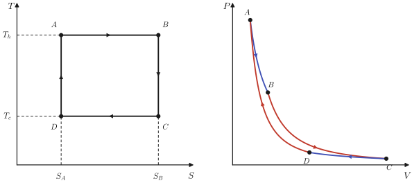
parameter; if the auxiliary system is a gas it may be caused to expand isothermally, if it is a magnetic system its magnetic moment may be decreased isothermally, and so forth. In this process a flux of heat occurs from the hot reservoir to the auxiliary system, and a transfer of work ( \(\int P d V\) or its magnetic or other analogue) occurs from the auxiliary system to the reversible work source. This is the isothermal step \(A \rightarrow B\) in Fig. 4.7. 2. The auxiliary system, now in contact only with the reversible work. source, is adiabatically expanded (or adiabatically demagnetized, etc.) until its temperature falls to that of the cold reservoir. A further transfer of work occurs from the auxiliary system to the reversible work source. The quasi-static adiabatic process occurs at constant entropy of the auxiliary system, as in \(B \rightarrow C\) of Fig. 4.7. 3. The auxiliary system is isothermally compressed while in contact with the cold reservoir and the reversible work source. This compression is continued until the entropy of the auxiliary system attains its initial value. During this process there is a transfer of work from the reversible work source to the auxiliary system, and a transfer of heat from the auxiliary system to the cold reservoir. This is the step \(C \rightarrow D\) in Fig. 4.7. 4. The auxiliary system is adiabatically compressed and receives work from the reversible work source. The compression brings the auxiliary system to its initial state and completes the cycle. Again the entropy of the auxiliary system is constant, from \(D\) to \(A\) in Fig. 4.7.
The heat withdrawn from the primary system (the hot reservoir) in process 1 is \(T_{h} \Delta S\), and the heat transferred to the cold reservoir in process 3 is \(T_{c} \Delta S\). The difference \(\left(T_{h}-T_{c}\right) \Delta S\) is the net work transferred to the reversible work source in the complete cycle. On the \(T-S\) diagram of Fig. 4.7 the heat \(T_{h} \Delta S\) withdrawn from the primary system is represented by the area bounded by the four points labeled \(A B S_{B} S_{A}\), the heat ejected to the cold reservoir is represented by the area \(C D S_{A} S_{B}\), and the net work delivered is represented by the area \(A B C D\). The coefficient of performance is the ratio of the area \(A B C D\) to the area \(A B S_{B} S_{A}\) or \(\left(T_{h}-T_{c}\right) / T_{h}\).
The Carnot cycle can be represented on any of a number of other diagrams, such as a \(P-V\) diagram or a \(T-V\) diagram. The representation on a \(P-V\) diagram is indicated in Fig. 4.7. The precise form of the curve \(B C\), representing the dependence of \(P\) on \(V\) in an adiabatic (isentropic) process, would follow from the equation of state \(P=P(S, V, N)\) of the auxiliary system.
If the hot and cold systems are merely reversible heat sources, rather than reservoirs, the Carnot cycle must be carried out in infinitesimal steps. The heat withdrawn from the primary (hot) system in process 1 is then \(T_{h} d S\) rather than \(T_{h} \Delta S\), and similarly for the other steps. There is clearly no difference in the essential results, although \(T_{h}\) and \(T_{c}\) are continually changing variables and the net evaluation of the process requires an integration over the differential steps.
It should be noted that real engines never attain ideal thermodynamic efficiency. Because of mechanical friction, and because they cannot be operated so slowly as to be truly quasi-static, they seldom attain more than 30 or 40% thermodynamic efficiency. Nevertheless, the upper limit on the efficiency, set by basic thermodynamic principles, is an important factor in engineering design. There are other factors as well, to which we shall return in Section 4.9.
Example
\(N\) moles of a monatomic ideal gas are to be employed as the auxiliary system in a Carnot cycle. The ideal gas is initially in contact with the hot reservoir, and in the first stage of the cycle it is expanded from volume \(V_{A}\) to volume \(V_{B} .{ }^{4}\) Calculate the work and heat transfers in each of the four steps of the cycle, in terms of \(T_{h}\), \(T_{c}, V_{A}, V_{B}\), and \(N\). Directly corroborate that the efficiency of the cycle is the Carnot efficiency.
Solution
The data are given in terms of \(T\) and \(V\); we therefore express the entropy and energy as functions of \(T, V\), and \(N\).
\[ S=N s_{0}+N R \ln \left(\frac{T^{3 / 2} V N_{0}}{T_{0}^{3 / 2} V_{0} N}\right) \]
and
\[ U=\frac{3}{2} N R T \]
Then in the isothermal expansion at temperature \(T_{h}\)
\[ \Delta S_{A B}=S_{B}-S_{A}=N R \ln \left(\frac{V_{B}}{V_{A}}\right) \text { and } \Delta U_{A B}=0 \]
[^10]whence \[ Q_{A B}=T_{h} \Delta S_{A B}=N R T_{h} \ln \left(\frac{V_{B}}{V_{A}}\right) \] and \[ W_{A B}=-N R T_{h} \ln \left(\frac{V_{B}}{V_{A}}\right) \]
In the second step of the cycle the gas is expanded adiabatically until the temperature falls to \(T_{c}\), the volume meanwhile increasing to \(V_{c}\). From the equation for \(S\), we see that \(T^{\frac{3}{2}} V=\) constant, and
\[ V_{C}=V_{B}\left(\frac{T_{h}}{T_{c}}\right)^{3 / 2} \]
and
\[ Q_{B C}=0 \quad W_{B C}=\Delta U=\frac{3}{2} N R\left(T_{c}-T_{h}\right) \]
In the third step the gas is isothermally compressed to a volume \(V_{D}\). This volume must be such that it lies on the same adiabat as \(V_{A}\) (see Fig. 4.7), so that
\[ V_{D}=V_{A}\left(\frac{T_{h}}{T_{c}}\right)^{3 / 2} \]
Then, as in step 1,
\[ Q_{C D}=N R T_{c} \ln \left(\frac{V_{D}}{V_{C}}\right)=N R T_{c} \ln \left(\frac{V_{A}}{V_{B}}\right) \]
and
\[ W_{C D}=-N R T_{c} \ln \left(\frac{V_{A}}{V_{B}}\right) \]
Finally, in the adiabatic compression
\[ Q_{D A}=0 \]
and
\[ W_{D A}=U_{D A}=\frac{3}{2} N R\left(T_{h}-T_{c}\right) \]
From these results we obtain
\[ W=W_{A B}+W_{B C}+W_{C D}+W_{D A}=-N R\left(T_{h}-T_{c}\right) \ln \left(\frac{V_{B}}{V_{A}}\right) \]
and
\[ -W / Q_{A B}=\left(T_{h}-T_{c}\right) / T_{h} \]
which is the expected Carnot efficiency.
PROBLEMS
Problem 4.7-1
Repeat the calculation of Example 5 assuming the “working substance” of the auxiliary system to be 1 mole of an ideal van der Waals fluid rather than of a monatomic ideal gas (recall Section 3.5).
Problem 4.7-2
Calculate the work and heat transfers in each stage of the Carnot cycle for the auxiliary system being an “empty” cylinder (containing only electromagnetic radiation). The first step of the cycle is again specified to be an expansion from \(V_{A}\) to \(V_{B}\). All results are to be expressed in terms of \(V_{A}, V_{B}, T_{h}\), and \(T_{c^{c}}\). Show that the ratio of the total work transfer to the first-stage heat transfer agrees with the Carnot efficiency.
Problem 4.7-3
A “primary subsystem” in the initial state \(A\) is to be brought reversibly to a specified final state \(B\). A reversible work source and a thermal reservoir at temperature \(T_{r}\) are available, but no “auxiliary system” is to be employed. Is it possible to devise such a process? Prove your answer. Discuss Problem 4.5-2 in this context.
Problem 4.7-4
The fundamental equation of a particular fluid is \(U N^{\frac{1}{2}} V^{\frac{3}{2}}=A(S-R)^{3}\) where \(A=2 \times 10^{-2}\left(\mathrm{~K}^{3} \mathrm{~m}^{\frac{9}{2}} / \mathrm{J}^{3}\right)\). Two moles of this fluid are used as the auxiliary system in a Carnot cycle, operating between two thermal reservoirs at temperature 100°C and 0°C. In the first isothermal expansion \(10^{6} \mathrm{~J}\) is extracted from the high-temperature reservoir. Find the heat transfer and the work transfer for each of the four processes in the Carnot cycle.
Calculate the efficiency of the cycle directly from the work and heat transfers just computed. Does this efficiency agree with the theoretical Carnot efficiency? Hint: Carnot cycle problems generally are best discussed in terms of a \(T-S\) diagram for the auxiliary system.
Problem 4.7-5
One mole of the “simple paramagnetic model system” of equation 3.66 is to be used as the auxiliary system of a Carnot cycle operating between reservoirs of temperature \(T_{h}\) and \(T_{c}\). The auxiliary system initially has a magnetic moment \(I_{t}\) and is at temperature \(T_{h}\). By decreasing the external field while the system is in contact with the high temperature reservoir, a quantity of heat \(Q_{1}\) is absorbed from the reservoir; the system meanwhile does work \(\left(-W_{1}\right)\) on the reversible work source (i.e., on the external system that creates the magnetic field and thereby induces the magnetic moment). Describe each step in the Carnot cycle and calculate the work and heat transfer in each step, expressing each in terms of \(T_{h}, T_{c}, Q_{1}\), and the parameters \(T_{0}\) and \(I_{0}\) appearing in the fundamental equation.
Problem 4.7-6
Repeat Problem 4.7-4 using the “rubber band” model of Section 3.7 as the auxiliary system.
PROBLEMS
Problem 4.8-1
To corroborate equation 4.22 show that
\[ \left(\frac{\partial P}{\partial s}\right)_{T}=-\left(\frac{\partial T}{\partial v}\right)_{P} \]
First consider the right-hand side, and write generally that
\[ d T=u_{s s} d s+u_{v s} d v \]
so that
\[ \left(\frac{\partial T}{\partial v}\right)_{P}=u_{s s}\left(\frac{\partial s}{\partial v}\right)_{P}+u_{v s}=-u_{s s} \frac{u_{v v}}{u_{s v}}+u_{v s} \]
Similarly show that \(\left(\frac{\partial P}{\partial s}\right)_{T}=u_{s s} u_{v v} / u_{s v}-u_{s v}\), establishing the required identity.
PROBLEMS
Problem 4.9-1
Show that the efficiency of an endoreversible engine, maximized for power output, is always less than \(\varepsilon_{\text {Carnot }}\). Plot the former efficiency as a function of the Carnot efficiency.
Problem 4.9-2
Suppose the conductance \(\sigma_{h}\left(=\sigma_{c}\right)\) to be such that 1 kW is transferred to the system (as heat flux) if its temperature is 50 K below that of the high temperature reservoir. Assuming \(T_{h}=800 \mathrm{~K}\) and \(T_{c}=300 \mathrm{~K}\), calculate the maximum power obtainable from an endoreversible engine, and find the temperatures \(T_{w}\) and \(T_{t}\) for which such an engine should be designed.
Problem 4.9-3
Consider an endoreversible engine for which the high temperature reservoir is boiling water \(\left(100^{\circ} \mathrm{C}\right)\) and the cold reservoir is at room temperature (taken as \(20^{\circ} \mathrm{C}\) ). Assuming the engine is operated at maximum power, what is the ratio of the amount of heat withdrawn from the high temperature reservoir (per kilowatt hour of delivered work) to that withdrawn by a Carnot engine? How much heat is withdrawn by each engine per kilowatt hour of delivered work?
Answer:
\[ \text { Ratio }=1.9 \]
Problem 4.9-4
Assume that one cycle of the engine of Problem 4.9-3 takes 20 s and that the conductance \(\sigma_{h}=\sigma_{c}=100 \mathrm{~W} / \mathrm{K}\). How much work is delivered per cycle? Assuming the “control volume” (i.e., the auxiliary system) is a gas, driven through a Carnot cycle, plot a \(T-S\) diagram of the gas during the cycle. Indicate numerical values for each vertex of the diagram (note that one value of the entropy can be assigned arbitrarily).
PROBLEMS
Problem 4.10-1
Assuming that the working gas is a monatomic ideal gas, plot a \(T-S\) diagram for the Otto cycle.
Problem 4.10-2
Assuming that the working gas is a simple ideal gas (with temperature independent heat capacities), show that the engine efficiency of the Otto cycle is given by equation 4.30.
Problem 4.10-3
Assuming that the working gas is a simple ideal gas (with temperature independent heat capacities), show that the engine efficiency of the Brayton cycle is given by equation 4.31.
Problem 4.10-4
Assuming that the working gas is a monatomic ideal gas, plot a \(T-S\) diagram of the Brayton cycle.
Problem 4.10-5
Assuming that the working gas is a monatomic ideal gas, plot a \(T-S\) diagram of the air-standard diesel cycle.