GENERAL PRINCIPLES OF CLASSICAL THERMODYNAMICS
INTRODUCTION
The Nature of Thermodynamics and the Basis of ThermoStatistics
Whether we are physicists, chemists, biologists, or engineers, our primary interface with nature is through the properties of macroscopic matter. Those properties are subject to universal regularities and to stringent limitations. Subtle relationships exist among apparently unconnected properties.
The existence of such an underlying order has far reaching implications. Physicists and chemists familiar with that order need not confront each new material as a virgin puzzle. Engineers are able to anticipate limitations to device designs predicated on creatively imagined (but yet undiscovered) materials with the requisite properties. And the specific form of the underlying order provides incisive clues to the structure of fundamental physical theory.
Certain primal concepts of thermodynamics are intuitively familiar. A metallic block released from rest near the rim of a smoothly polished metallic bowl oscillates within the bowl, approximately conserving the sum of potential and kinetic energies. But the block eventually comes to rest at the bottom of the bowl. Although the mechanical energy appears to have vanished, an observable effect is wrought upon the material of the bowl and block; they are very slightly, but perceptibly, “warmer.” Even before studying thermodynamics, we are qualitatively aware that the mechanical energy has merely been converted to another form, that the fundamental principle of energy conservation is preserved, and that the physiological sensation of “warmth” is associated with the thermodynamic concept of “temperature.”
Vague and undefined as these observations may be, they nevertheless reveal a notable dissimilarity between thermodynamics and the other branches of classical science. Two prototypes of the classical scientific paradigm are mechanics and electromagnetic theory. The former addresses itself to the dynamics of particles acted upon by forces, the latter to the dynamics of the fields that mediate those forces. In each of these cases a new “law” is formulated-for mechanics it is Newton’s Law (or Lagrange or Hamilton’s more sophisticated variants); for electromagnetism it is the Maxwell equations. In either case it remains only to explicate the consequences of the law.
Thermodynamics is quite different. It neither claims a unique domain of systems over which it asserts primacy, nor does it introduce a new fundamental law analogous to Newton’s or Maxwell’s equations. In contrast to the specificity of mechanics and electromagnetism, the hallmark of thermodynamics is generality. Generality first in the sense that thermodynamics applies to all types of systems in macroscopic aggrega- tion, and second in the sense that thermodynamics does not predict specific numerical values for observable quantities. Instead, thermodynamics sets limits (inequalities) on permissible physical processes, and it establishes relationships among apparently unrelated properties.
The contrast between thermodynamics and its counterpart sciences raises fundamental questions which we shall address directly only in the final chapter. There we shall see that whereas thermodynamics is not based on a new and particular law of nature, it instead reflects a commonality or universal feature of all laws. In brief, thermodynamics is the study of the restrictions on the possible properties of matter that follow from the symmetry properties of the fundamental laws of physics.
The connection between the symmetry of fundamental laws and the macroscopic properties of matter is not trivially evident, and we do not attempt to derive the latter from the former. Instead we follow the postulatory formulation of thermodynamics developed in the first edition of this text, returning to an interpretive discussion of symmetry origins in Chapter 21. But even the preliminary assertion of this basis of thermodynamics may help to prepare the reader for the somewhat uncommon form of thermodynamic theory. Thermodynamics inherits its universality, it nonmetric nature, and its emphasis on relationships from its symmetry parentage. \(12\)
THE PROBLEM AND THE POSTULATES
1-1 THE TEMPORAL NATURE OF MACROSCOPIC MEASUREMENTS
Perhaps the most striking feature of macroscopic matter is the incredible simplicity with which it can be characterized. We go to a pharmacy and request one liter of ethyl alcohol, and that meager specification is pragmatically sufficient. Yet from the atomistic point of view, we have specified remarkably little. A complete mathematical characterization of the system would entail the specification of coordinates and momenta for each molecule in the sample, plus sundry additional variables descriptive of the internal state of each molecule-altogether at least \(10^{23}\) numbers to describe the liter of alcohol! A computer printing one coordinate each microsecond would require 10 billion years-the age of the universe-to list the atomic coordinates. Somehow, among the \(10^{23}\) atomic coordinates, or linear combinations of them, all but a few are macroscopically irrelevant. The pertinent few emerge as macroscopic coordinates, or “thermodynamic coordinates.”
Like all sciences, thermodynamics is a description of the results to be obtained in particular types of measurements. The character of the contemplated measurements dictates the appropriate descriptive variables; these variables, in turn, ordain the scope and structure of thermodynamic theory.
The key to the simplicity of macroscopic description, and the criterion for the choice of thermodynamic coordinates, lies in two attributes of macroscopic measurement. Macroscopic measurements are extremely slow on the atomic scale of time, and they are extremely coarse on the atomic scale of distance.
While a macroscopic measurement is being made, the atoms of a system go through extremely rapid and complex motions. To measure the length of a bar of metal we might choose to calibrate it in terms of the wavelength of yellow light, devising some arrangement whereby reflection from the end of the bar produces interference fringes. These fringes are then to be photographed and counted. The duration of the measurement is determined by the shutter speed of the camera-typically on the order of one hundredth of a second. But the characteristic period of vibration of the atoms at the end of the bar is on the order of \(10^{-15}\) seconds!
A macroscopic observation cannot respond to those myriads of atomic coordinates which vary in time with typical atomic periods. Only those few particular combinations of atomic coordinates that are essentially time independent are macroscopically observable.
The word essentially is an important qualification. In fact we are able to observe macroscopic processes that are almost, but not quite, time independent. With modest difficulty we might observe processes with time scales on the order of \(10^{-7} \mathrm{~s}\) or less. Such observable processes are still enormously slow relative to the atomic scale of \(10^{-15} \mathrm{~s}\). It is rational then to first consider the limiting case and to erect a theory of time-independent phenomena. Such a theory is thermodynamics.
By definition, suggested by the nature of macroscopic observations, thermodynamics describes only static states of macroscopic systems.
Of all the \(10^{23}\) atomic coordinates, or combinations thereof, only a few are time independent.
Quantities subject to conservation principles are the most obvious candidates as time-independent thermodynamic coordinates: the energy, each component of the total momentum, and each component of the total angular momentum of the system. But there are other time-independent thermodynamic coordinates, which we shall enumerate after exploring the spatial nature of macroscopic measurement.
1-2 THE SPATIAL NATURE OF MACROSCOPIC MEASUREMENTS
Macroscopic measurements are not only extremely slow on the atomic scale of time, but they are correspondingly coarse on the atomic scale of distance. We probe our system always with “blunt instruments.” Thus an optical observation has a resolving power defined by the wavelength of light, which is on the order of 1000 interatomic distances. The smallest resolvable volume contains approximately \(10^{9}\) atoms! Macroscopic observations sense only coarse spatial averages of atomic coordinates.
The two types of averaging implicit in macroscopic observations together effect the enormous reduction in the number of pertinent variables, from the initial \(10^{23}\) atomic coordinates to the remarkably small number of thermodynamic coordinates. The manner of reduction can be illustrated schematically by considering a simple model system, as shown in Fig. 1.1. The model system consists not of \(10^{23}\) atoms, but of only 9. These atoms are spaced along a one-dimensional line, are constrained to
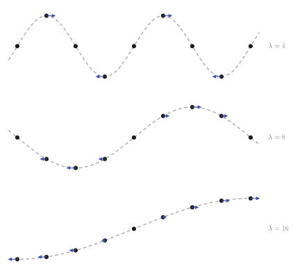
move only along that line, and interact by linear forces (as if connected by springs). The motions of the individual atoms are strongly coupled, so the atoms tend to move in organized patterns called normal modes. Three such normal modes of motion are indicated schematically in Fig. 1.1. The arrows indicate the displacements of the atoms at a particular moment; the atoms oscillate back and forth, and half a cycle later all the arrows would be reversed.
Rather than describe the atomic state of the system by specifying the position of each atom, it is more convenient (and mathematically equivalent) to specify the instantaneous amplitude of each normal mode. These amplitudes are called normal coordinates, and the number of normal coordinates is exactly equal to the number of atomic coordinates.
In a “macroscopic” system composed of only nine atoms there is no precise distinction between “macroscopic” and “atomic” observations. For the purpose of illustration, however, we think of a macroscopic observation as a kind of “blurred” observation with low resolving power; the spatial coarseness of macroscopic measurements is qualitatively analogous to visual observation of the system through spectacles that are somewhat out of focus. Under such observation the fine structure of the first two modes in Fig. 1.1 is unresolvable, and these modes are rendered unobservable and macroscopically irrelevant. The third mode, however, corresponds to a relatively homogeneous net expansion (or contraction) of the whole system. Unlike the first two modes, it is easily observable through “blurring spectacles.” The amplitude of this mode describes the length (or volume, in three dimensions) of the system. The length (or volume) remains as a thermodynamic variable, undestroyed by the spatial averaging, because of its spatially homogeneous (long wavelength) structure.
The time averaging associated with macroscopic measurements augments these considerations. Each of the normal modes of the system has a characteristic trequency, the frequency being smaller for modes of longer wavelength. The frequency of the third normal mode in Fig. 1.1 is the lowest of those shown, and if we were to consider systems with very large numbers of atoms, the frequency of the longest wavelength mode would approach zero (for reasons to be explored more fully in Chapter 21). Thus all the short wavelength modes are lost in the time averaging, but the long wavelength mode corresponding to the “volume” is so slow that it survives the time averaging as well as the spatial averaging.
This simple example illustrates a very general result. Of the enormous number of atomic coordinates, a very few, with unique symmetry properties, survive the statistical averaging associated with a transition to a macroscopic description. Certain of these surviving coordinates are mechanical in nature-they are volume, parameters descriptive of the shape (components of elastic strain), and the like. Other surviving coordinates are electrical in nature-they are electric dipole moments, magnetic dipole moments, various multipole moments, and the like. The study of mechanics (including elasticity) is the study of one set of surviving coordinates. The subject of electricity (including electrostatics, magnetostatics, and ferromagnetism) is the study of another set of surviving coordinates.
Thermodynamics, in contrast, is concerned with the macroscopic consequences of the myriads of atomic coordinates that, by virtue of the coarseness of macroscopic observations, do not appear explicitly in a macroscopic description of a system.
Among the many consequences of the “hidden” atomic modes of motion, the most evident is the ability of these modes to act as a repository for energy. Energy transferred via a “mechanical mode” (i.e., one associated with a mechanical macroscopic coordinate) is called mechanical work. Energy transferred via an “electrical mode” is called electrical work. Mechanical work is typified by the term \(-P d V\) ( \(P\) is pressure, \(V\) is volume), and electrical work is typified by the term \(-E_{e} d \mathscr{P}\) ( \(E_{e}\) is electric field, \(\mathscr{P}\) is electric dipole moment). These energy terms and various other mechanical and electrical work terms are treated fully in the standard mechanics and electricity references. But it is equally possible to transfer energy via the hidden atomic modes of motion as well as via those that happen to be macroscopically observable. An energy transfer via .he hidden atomic modes is called heat. Of course this descriptive characterization of heat is not a sufficient basis for the formal development of thermodynamics, and we shall soon formulate an appropriate operational definition.
With this contextual perspective we proceed to certain definitions and conventions needed for the theoretical development.
1-3 THE COMPOSITION OF THERMODYNAMIC SYSTEMS
Thermodynamics is a subject of great generality, applicable to systems of elaborate structure with all manner of complex mechanical, electrical, and thermal properties. We wish to focus our chief attention on the thermal properties. Therefore it is convenient to idealize and simplify the mechanical and electrical properties of the systems that we shall study initially. Similarly, in mechanics we consider uncharged and unpolarized systems; whereas in electricity we consider systems with no elastic compressibility or other mechanical attributes. The generality of either subject is not essentially reduced by this idealization, and after the separate content of each subject has been studied it is a simple matter to combine the theories to treat systems of simultaneously complicated electrical and mechanical properties. Similarly, in our study of thermodynamics we idealize our systems so that their mechanical and electrical properties are almost trivially simple. When the essential content of thermodynamics has thus been developed, it again is a simple matter to extend the analysis to systems with relatively complex mechanical and electrical structure. The essential point to be stressed is that the restrictions on the types of systems considered in the following several chapters are not basic limitations on the generality of thermodynamic theory but are adopted merely for simplicity of exposition.
We (temporarily) restrict our attention to simple systems, defined as systems that are macroscopically homogeneous, isotropic, and uncharged, that are large enough so that surface effects can be neglected, and that are not acted on by electric, magnetic, or gravitational fields.
For such a simple system there are no macroscopic electric coordinates whatsoever. The system is uncharged and has neither electric nor magnetic dipole, quadrupole, or higher-order moments. All elastic shear components and other such mechanical parameters are zero. The volume \(V\) does remain as a relevant mechanical parameter. Furthermore, a simple system has a definite chemical composition which must be described by an appropriate set of parameters. One reasonable set of composition parameters is the numbers of molecules in each of the chemically pure components of which the system is a mixture. Alternatively, to obtain numbers of more convenient size, we adopt the mole numbers, defined as the actual number of each type of molecule divided by Avogadro’s number ( \(\mathrm{N}_{\mathrm{A}}=\) \(6.02217 \times 10^{23}\) ).
This definition of the mole number refers explicitly to the “number of molecules,” and it therefore lies outside the boundary of purely macroscopic physics. An equivalent definition which avoids the reference to molecules simply designates 12 grams as the molar mass of the isotope \({ }^{12} \mathrm{C}\). The molar masses of other isotopes are then defined to stand in the same ratio as the conventional “atomic masses,” a partial list of which is given in Table 1.1.
TABLE 1.1 Atomic Masses (g) of Some Naturally Occurring Elements (Mixtures of Isotopes) \({ }^{a}\)
| H | 1.0080 | F | 18.9984 |
|---|---|---|---|
| Li | 6.941 | Na | 22.9898 |
| C | 12.011 | Al | 26.9815 |
| N | 14.0067 | S | 32.06 |
| O | 15.9994 | Cl | 35.453 |
\({ }^{a}\) As adopted by the International Union of Pure and Applied Chemistry, 1969.
If a system is a mixture of \(r\) chemical components, the \(r\) ratios \(N_{k} /\left(\sum_{j=1}^{r} N_{j}\right)(k=1,2, \ldots, r)\) are called the mole fractions. The sum of all \(r\) mole fractions is unity. The quantity \(V /\left(\sum_{\mathrm{j}=1}^{r} N_{j}\right)\) is called the molar volume.
The macroscopic parameters \(V, N_{1}, N_{2}, \ldots, N_{r}\) have a common property that will prove to be quite significant. Suppose that we are given two identical systems and that we now regard these two systems taken together as a single system. The value of the volume for the composite system is then just twice the value of the volume for a single subsystem. Similarly, each of the mole numbers of the composite system is twice that for a single subsystem. Parameters that have values in a composite system equal to the sum of the values in each of the subsystems are called extensive parameters. Extensive parameters play a key role throughout thermodynamic theory.
PROBLEMS
Problem 1.3-1
One tenth of a kilogram of NaCl and 0.15 kg of sugar \(\left(\mathrm{C}_{12} \mathrm{H}_{22} \mathrm{O}_{11}\right)\) are dissolved in 0.50 kg of pure water. The volume of the resultant thermodynamic system is \(0.55 \times 10^{-3} \mathrm{~m}^{3}\). What are the mole numbers of the three components of the system? What are the mole fractions? What is the molar volume of the system? It is sufficient to carry the calculations only to two significant figures.
Answer: Mole fraction of \(\mathrm{NaCl}=0.057\); molar volume \(=18 \times 10^{-6} \mathrm{~m}^{3} /\) mole .
Problem 1.3-2
Naturally occurring boron has an atomic mass of 10.811 g . It is a mixture of the isotopes \({ }^{10} \mathrm{~B}\) with an atomic mass of 10.0129 g and \({ }^{11} \mathrm{~B}\) with an atomic mass of 11.0093 g . What is the mole fraction of \({ }^{10} \mathrm{~B}\) in the mixture?
Problem 1.3-3
Twenty cubic centimeters each of ethyl alcohol \(\left(\mathrm{C}_{2} \mathrm{H}_{5} \mathrm{OH}\right.\); density \(=0.79\) \(\left.\mathrm{g} / \mathrm{cm}^{3}\right)\), methyl alcohol \(\left(\mathrm{CH}_{3} \mathrm{OH}\right.\); density \(\left.=0.81 \mathrm{~g} / \mathrm{cm}^{3}\right)\), and water \(\left(\mathrm{H}_{3} \mathrm{O}\right.\) :
density \(=1 \mathrm{~g} / \mathrm{cm}^{3}\) ) are mixed together. What are the mole numbers and mole fractions of the three components of the system?
Answer:
\[ \text { mole fractions }=0.17,0.26,0.57 \]
Problem 1.3-4
A 0.01 kg sample is composed of 50 molecular percent \(\mathrm{H}_{2}\), 30 molecular percent HD (hydrogen deuteride), and 20 molecular percent \(\mathrm{D}_{2}\). What additional mass of \(D_{2}\) must be added if the mole fraction of \(D_{2}\) in the final mixture is to be 0.3?
Problem 1.3-5
A solution of sugar \(\left(\mathrm{C}_{12} \mathrm{H}_{22} \mathrm{O}_{11}\right)\) in water is 20% sugar by weight. What is the mole fraction of sugar in the solution?
Problem 1.3-6
An aqueous solution of an unidentified solute has a total mass of 0.1029 kg. The mole fraction of the solute is 0.1. The solution is diluted with 0.036 kg of water, after which the mole fraction of the solute is 0.07. What would be a reasonable guess as to the chemical identity of the solute?
Problem 1.3-7
One tenth of a kg of an aqueous solution of HCl is poured into 0.2 kg of an aqueous solution of NaOH. The mole fraction of the HCl solution was 0.1 , whereas that of the NaOH solution was 0.25 . What are the mole fractions of each of the components in the solution after the chemical reaction has come to completion?
Answer:
\[ x_{\mathrm{H}_{2} \mathrm{O}}=N_{\mathrm{H}_{2} \mathrm{O}} / N=0.84 \]
1-4 THE INTERNAL ENERGY
The development of the principle of conservation of energy has been one of the most significant achievements in the evolution of physics. The present form of the principle was not discovered in one magnificent stroke of insight but was slowly and laboriously developed over two and a half centuries. The first recognition of a conservation principle, by Leibniz in 1693, referred orily to the sum of the kinetic energy ( \(\frac{1}{2} m v^{2}\) ) and the potential energy (mgh) of a simple mechanical mass point in the terrestrial gravitational field. As additional types of systems were considered the established form of the conservation principle repeatedly failed, but in each case it was found possible to revive it by the addition of a new mathematical term-a “new kind of energy.” Thus consideration of charged systems necessitated the addition of the Coulomb interaction energy ( \(Q_{1} Q_{2} / r\) ) and eventually of the energy of the electromagnetic field. In 1905 Einstein extended the principle to the relativistic region, adding such terms as the relativistic rest-mass energy. In the 1930s Enrico Fermi postulated the existence of purpose of retaining the energy conservation principle in nuclear reactions. The principle of energy conservation is now seen as a reflection of the (presumed) fact that the fundamental laws of physics are the same today as they were eons ago, or as they will be in the remote future; the laws of physics are unaltered by a shift in the scale of time ( \(t \rightarrow t+\) constant). Of this basis for energy conservation we shall have more to say in Chapter 21. Now we simply note that the energy conservation principle is one of the most fundamental, general, and significant principles of physical theory.
Viewing a macroscopic system as an agglomerate of an enormous number of electrons and nuclei, interacting with complex but definite forces to which the energy conservation principle applies, we conclude that macroscopic systems have definite and precise energies, subject to a definite conservation principle. That is, we now accept the existence of a well-defined energy of a thermodynamic system as a macroscopic manifestation of a conservation law, highly developed, tested to an extreme precision, and apparently of complete generality at the atomic level.
The foregoing justification of the existence of a thermodynamic energy function is quite different from the historical thermodynamic method. Because thermodynamics was developed largely before the atomic hypothesis was accepted, the existence of a conservative macroscopic energy function had to be demonstrated by purely macroscopic means. A significant step in that direction was taken by Count Rumford in 1798 as he observed certain thermal effects associated with the boring of brass cannons. Sir Humphry Davy, Sadi Carnot, Robert Mayer, and, finally (between 1840 and 1850), James Joule carried Rumford’s initial efforts to their logical fruition. The history of the concept of heat as a form of energy transfer is unsurpassed as a case study in the tortuous development of scientific theory, as an illustration of the almost insuperable inertia presented by accepted physical doctrine, and as a superb tale of human ingenuity applied to a subtle and abstract problem. The interested reader is referred to The Early Development of the Concepts of Temperature and Heat by D. Roller (Harvard University Press, 1950) or to any standard work on the history of physics.
Although we shall not have recourse explicitly to the experiments of Rumford and Joule in order to justify our postulate of the existence of an energy function, we make reference to them in Section 1.7 in our discussion of the measurability of the thermodynamic energy.
Only differences of energy, rather than absolute values of the energy, have physical significance, either at the atomic level or in macroscopic systems. It is conventional therefore to adopt some particular state of a system as a fiducial state, the energy of which is arbitrarily taken as zero. The energy of a system in any other state, relative to the energy of the system in the fiducial state, is then called the thermodynamic internal energy of the system in that state and is denoted by the symbol U. Like the volume and the mole numbers, the internal energy is an extensive parameter.
1-5 THERMODYNAMIC EQUILIBRIUM
Macroscopic systems often exhibit some “memory” of their recent history. A stirred cup of tea continues to swirl within the cup. Cold-worked steel maintains an enhanced hardness imparted by its mechanical treatment. But memory eventually fades. Turbulences damp out, internal strains yield to plastic flow, concentration inhomogeneities diffuse to uniformity. Systems tend to subside to very simple states, independent of their specific history.
In some cases the evolution toward simplicity is rapid; in other cases it can proceed with glacial slowness. But in all systems there is a tendency to evolve toward states in which the properties are determined by intrinsic factors and not by previously applied external influences. Such simple terminal states are, by definition, time independent. They are called equilibrium states.
Thermodynamics seeks to describe these simple, static “equilibrium” states to which systems eventually evolve.
To convert this statement to a formal and precise postulate we first recognize that an appropriate criterion of simplicity is the possibility of description in terms of a small number of variables. It therefore seems plausible to adopt the following postulate, suggested by experimental observation and formal simplicity, and to be verified ultimately by the success of the derived theory:
Postulate I. There exist particular states (called equilibrium states) of simple systems that, macroscopically, are characterized completely by the internal energy \(U\), the volume \(V\), and the mole numbers \(N_{1}, N_{2}, \ldots, N_{r}\) of the chemical components.
As we expand the generality of the systems to be considered, eventually permitting more complicated mechanical and electrical properties, the number of parameters required to characterize an equilibrium state increases to include, for example, the electric dipole moment and certain elastic strain parameters. These new variables play roles in the formalism which are completely analogous to the role of the volume \(V\) for a simple system.
A persistent problem of the experimentalist is to determine somehow whether a given system actually is in an equilibrium state, to which thermodynamic analysis can be applied. He or she can, of course, observe whether the system is static and quiescent. But quiescence is not sufficient. As the state is assumed to be characterized completely by the extensive parameters, \(U, V, N_{1}, N_{2}, \ldots, N_{r}\), it follows that the properties of the system must be independent of the past history. This is hardly an operational prescription for the recognition of an equilibrium state, but in certain cases this independence of the past history is obviously not satisfied, and these cases give some insight into the significance of equilibrium. Thus two pieces of chemically identical commercial steel may have very different properties imparted by cold-working, heat treatment, quenching, and annealing in the manufacturing process. Such systems are clearly not in equilibrium. Similarly, the physical characteristics of glass depend upon the cooling rate and other details of its manufacture; hence glass is not in equilibrium.
If a system that is not in equilibrium is analyzed on the basis of a thermodynamic formalism predicated on the supposition of equilibrium, inconsistencies appear in the formalism and predicted results are at variance with experimental observations. This failure of the theory is used by the experimentalist as an a posteriori criterion for the detection of nonequilibrium states.
In those cases in which an unexpected inconsistency arises in the thermodynamic formalism a more incisive quantum statistical theory usually provides valid reasons for the failure of the system to attain equilibrium. The occasional theoretical discrepancies that arise are therefore of great heuristic value in that they call attention to some unsuspected complication in the molecular mechanisms of the system. Such circumstances led to the discovery of ortho- and parahydrogen, \({ }^{1}\) and to the understanding of the molecular mechanism of conversion between the two forms.
From the atomic point of view, the macroscopic equilibrium state is associated with incessant and rapid transitions among all the atomic states consistent with the given boundary conditions. If the transition mechanism among the atomic states is sufficiently effective, the system passes rapidly through all representative atomic states in the course of a macroscopic observation; such a system is in equilibrium. However, under certain unique conditions, the mechanism of atomic transition may be ineffective and the system may be trapped in a small subset of atypical atomic states. Or even if the system is not completely trapped the rate of transition may be so slow that a macroscopic measurement does not yield a proper average over all possible atomic states. In these cases the system is not in equilibrium. It is readily apparent that such situations are most likely to occur in solid rather than in fluid systems, for the comparatively high atomic mobility in fluid systems and the random nature of the
[^0]interatomic collisions militate strongly against any restrictions of the atomic transition probabilities.
In actuality, few systems are in absolute and true equilibrium. In absolute equilibrium all radioactive materials would have decayed completely and nuclear reactions would have transmuted all nuclei to the most stable of isotopes. Such processes, which would take cosmic times to complete, generally can be ignored. A system that has completed the relevant processes of spontaneous evolution, and that can be described by a reasonably small number of parameters, can be considered to be in metastable equilibrium. Such a limited equilibrium is sufficient for the application of thermodynamics.
In practice the criterion for equilibrium is circular. Operationally, a system is in an equilibrium state if its properties are consistently described by thermodynamic theory!
It is important to reflect upon the fact that the circular character of thermodynamics is not fundamentally different from that of mechanics. A particle of known mass in a known gravitational field might be expected to move in a specific trajectory; if it does not do so we do not reject the theory of mechanics, but we simply conclude that some additional force acts on the particle. Thus the existence of an electrical charge on the particle, and the associated relevance of an electrical force, cannot be known a priori. It is inferred only by circular reasoning, in that dynamical predictions are incorrect unless the electric contribution to the force is included. Our model of a mechanical system (including the assignment of its mass, moment of inertia, charge, dipole moment, etc.) is “correct” if it yields successful predictions.
1-6 WALLS AND CONSTRAINTS
A description of a thermodynamic system requires the specification of the “walls” that separate it from the surroundings and that provide its boundary conditions. It is by means of manipulations of the walls that the extensive parameters of the system are altered and processes are initiated.
The processes arising by manipulations of the walls generally are associated with a redistribution of some quantity among various systems or among various portions of a single system. A formal classification of thermodynamic walls accordingly can be based on the property of the walls in permitting or preventing such redistributions. As a particular illustration, consider two systems separated by an internal piston within a closed, rigid cylinder. If the position of the piston is rigidly fixed the “wall” prevents the redistribution of volume between the two systems, but if the piston is left free such a redistribution is permitted. The cylinder and the rigidly fixed piston may be said to constitute a wall restrictive with respect to the volume, whereas the cylinder and the movable piston may be said to constitute a wall nonrestrictive with respect to the volume. In general, a wall that constrains an extensive parameter of a system to have a definite and particular value is said to be restrictive with respect to that parameter, whereas a wall that permits the parameter to change freely is said to be nonrestrictive with respect to that parameter.
A wall that is impermeable to a particular chemical component is restrictive with respect to the corresponding mole number; whereas a permeable membrane is nonrestrictive with respect to the mole number. Semipermeable membranes are restrictive with respect to certain mole numbers and nonrestrictive with respect to others. A wall with holes in it is nonrestrictive with respect to all mole numbers.
The existence of walls that are restrictive with respect to the energy is associated with the larger problem of measurability of the energy, to which we now turn our attention.
1-7 MEASURABILITY OF THE ENERGY
On the basis of atomic considerations, we have been led to accept the existence of a macroscopic conservative energy function. In order that this energy function may be meaningful in a practical sense, however, we must convince ourselves that it is macroscopically controllable and measurable. We shall now show that practical methods of measurement of the energy do exist, and in doing so we shall also be led to a quantitative operational definition of heat.
An essential prerequisite for the measurability of the energy is the existence of walls that do not permit the transfer of energy in the form of heat. We briefly examine a simple experimental situation that suggests that such walls do indeed exist.
Consider a system of ice and water enclosed in a container. We find that the ice can be caused to melt rapidly by stirring the system vigorously. By stirring the system we are clearly transferring energy to it mechanically, so that we infer that the melting of the ice is associated with an input of energy to the system. If we now observe the system on a summer day, we find that the ice spontaneously melts despite the fact that no work is done on the system. It therefore seems plausible that energy is being transferred to the system in the form of heat. We further observe that the rate of melting of the ice is progressively decreased by changing the wall surrounding the system from thin metal sheet, to thick glass, and thence to a Dewar wall (consisting of two silvered glass sheets separated by an evacuated interspace). This observation strongly suggests that the metal, glass, and Dewar walls are progressively less permeable to the flow of heat. The ingenuity of experimentalists has produced walls that are able to reduce the melting rate of the ice to a negligible value, and such walls are correspondingly excellent approximations to the limiting idealization of a wall that is truly impermeable to the flow of heat.
It is conventional to refer to a wall that is impermeable to the flow of heat as adiabatic; whereas a wall that permits the flow of heat is termed diathermal. If a wall allows the flux of neither work nor heat, it is restrictive with respect to the energy. A system enclosed by a wall that is restrictive with respect to the energy, volume, and all the mole numbers is said to be closed. \({ }^{2}\)
The existence of these several types of walls resolves the first of our concerns with the thermodynamic energy. That is, these walls demonstrate that the energy is macroscopically controllable. It can be trapped by restrictive walls and manipulated by diathermal walls. If the energy of a system is measured today, and if the system is enclosed by a wall restrictive with respect to the energy, we can be certain of the energy of the system tomorrow. Without such a wall the concept of a macroscopic thermodynamic energy would be purely academic.
We can now proceed to our second concern-that of measurability of the energy. More accurately, we are concerned with the measurability of energy differences, which alone have physical significance. Again we invoke the existence of adiabatic walls, and we note that for a simple system enclosed by an impermeable adiabatic wall the only type of permissible energy transfer is in the form of work. The theory of mechanics provides us with quantitative formulas for its measurement. If the work is done by compression, displacing a piston in a cylinder, the work is the product of force times displacement; or if the work is done by stirring, it is the product of the torque times the angular rotation of the stirrer shaft. In either case, the work is well defined and measurable by the theory of mechanics. We conclude that we are able to measure the energy difference of two states provided that one state can be reached from the other by some mechanical process while the system is enclosed by an adiabatic impermeable wall.
The entire matter of controllability and measurability of the energy can be succinctly stated as follows: There exist walls, called adiabatic, with the property that the work done in taking an adiabatically enclosed system between two given states is determined entirely by the states, independent of all external conditions. The work done is the difference in the internal energy of the two states.
As a specific example suppose we are given an equilibrium system composed of ice and water enclosed in a rigid adiabatic impermeable wall. Through a small hole in this wall we pass a thin shaft carrying a propellor blade at the inner end and a crank handle at the outer end. By turning the crank handle we can do work on the system. The work done is equal to the angular rotation of the shaft multiplied by the viscous torque. After turning the shaft for a definite time the system is allowed to come to a new equilibrium state in which some definite amount of the ice is observed
[^1]to have been melted. The difference in energy of the final and initial states is equal to the work that we have done in turning the crank.
We now inquire about the possibility of starting with some arbitrary given state of a system, of enclosing the system in an adiabatic impermeable wall, and of then being able to contrive some mechanical process that will take the system to another arbitrarily specified state. To determine the existence of such processes, we must have recourse to experimental observation, and it is here that the great classical experiments of Joule are relevant. His work can be interpreted as demonstrating that for a system enclosed by an adiabatic impermeable wall any two equilibrium states with the same set of mole numbers \(N_{1}, N_{2}, \ldots, N_{r}\) can be joined by some possible mechanical process. Joule discovered that if two states (say \(A\) and \(B\) ) are specified it may not be possible to find a mechanical process (consistent with an adiabatic impermeable wall) to take the system from \(A\) to \(B\) but that it is always possible to find either a process to take the system from \(A\) to \(B\) or a process to take the system from \(B\) to \(A\). That is, for any states \(A\) and \(B\) with equal mole numbers, either the adiabatic mechanical process \(A \rightarrow B\) or \(B \rightarrow A\) exists. For our purposes either of these processes is satisfactory. Experiment thus shows that the methods of mechanics permit us to measure the energy difference of any two states with equal mole numbers.
Joule’s observation that only one of the processes \(A \rightarrow B\) or \(B \rightarrow A\) may exist is of profound significance. This asymmetry of two given states is associated with the concept of irreversibility, with which we shall subsequently be much concerned.
The only remaining limitation to the measurability of the energy difference of any two states is the requirement that the states must have equal mole numbers. This restriction is easily eliminated by the following observation. Consider two simple subsystems separated by an impermeable wall and assume that the energy of each subsystem is known (relative to appropriate fiducial states, of course). If the impermeable wall is removed, the subsystems will intermix, but the total energy of the composite system will remain constant. Therefore the energy of the final mixed system is known to be the sum of the energies of the original subsystems. This technique enables us to relate the energies of states with different mole numbers.
In summary, we have seen that by employing adiabatic walls and by measuring only mechanical work, the energy of any thermodynamic system, relative to an appropriate reference state, can be measured.
1-8 QUANTITATIVE DEFINITION OF HEAT-UNITS
The fact that the energy difference of any two equilibrium states is measurable provides us directly with a quantitative definition of the heat: The heat flux to a system in any process (at constant mole numbers) is simply the difference in internal energy between the final and initial states, diminished by the work done in that process.
Consider some specified process that takes a system from the initial state \(A\) to the final state \(B\). We wish to know the amount of energy transferred to the system in the form of work and the amount transferred in the form of heat in that particular process. The work is easily measured by the method of mechanics. Furthermore, the total energy difference \(U_{B}-U_{A}\) is measurable by the procedures discussed in Section 1.7. Subtracting the work from the total energy difference gives us the heat flux in the specified process.
It should be noted that the amount of work associated with different processes may be different, even though each of the processes initiates in the same state \(A\) and each terminates in the same state \(B\). Similarly, the heat flux may be different for each of the processes. But the sum of the work and heat fluxes is just the total energy difference \(U_{B}-U_{A}\) and is the same for each of the processes. In referring to the total energy flux we therefore need specify only the initial and terminal states, but in referring to heat or work fluxes we must specify in detail the process considered.
Restricting our attention to thermodynamic simple systems, the quasistatic work is associated with a change in volume and is given quantitatively by
\[ d W_{M}=-P d V \]
where \(P\) is the pressure. In recalling this equation from mechanics, we stress that the equation applies only to quasi-static processes. A precise definition of quasi-static processes will be given in Section 4.2, but now we merely indicate the essential qualitative idea of such processes. Let us suppose that we are discussing, as a particular system, a gas enclosed in a cylinder fitted with a moving piston. If the piston is pushed in very rapidly, the gas immediately behind the piston acquires kinetic energy and is set into turbulent motion and the pressure is not well defined. In such a case the work done on the system is not quasi-static and is not given by equation 1.1. If, however, the piston is pushed in at a vanishingly slow rate (quasi-statically), the system is at every moment in a quiescent equilibrium state, and equation 1.1 then applies. The “infinite slowness” of the process is, roughly, the essential feature of a quasi-static process.
A second noteworthy feature of equation 1.1 is the sign convention. The work is taken to be positive if it increases the energy of the system. If the volume of the system is decreased, work is done on the system, increasing its energy; hence the negative sign in equation 1.1.
With the quantitative expression \(d W_{M}=-P d V\) for the quasi-static work, we can now give a quantitative expression for the heat flux. In an infinitesimal quasi-static process at constant mole numbers the quasi-static heat \(d Q\) is defined by the equation
\[ d Q=d U-d W_{M} \text { at constant mole numbers } \]
or
\[ d Q=d U+P d V \quad \text { at constant mole numbers } \]
It will be noted that we use the terms heat and heat flux interchangeably. Heat, like work, is only a form of energy transfer. Once energy is transferred to a system, either as heat or as work, it is indistinguishable from energy that might have been transferred differently. Thus, although \(d Q\) and \(d W_{M}\) add together to give \(d U\), the energy \(U\) of a state cannot be considered as the sum of “work” and “heat” components. To avoid this implication we put a stroke through the symbol \(d\) : infinitesimals such as \(d W_{M}\) and \(d Q\) are called imperfect differentials. The integrals of \(d W_{M}\) and \(d Q\) for a particular process are the work and heat fluxes in that process; the sum is the energy difference \(\Delta U\), which alone is independent of the process.
The concepts of heat, work, and energy may possibly be clarified in terms of a simple analogy. A certain farmer owns a pond, fed by one stream and drained by another. The pond also receives water from an occasional rainfall and loses it by evaporation, which we shall consider as “negative rain.” In this analogy the pond is our system, the water within it is the internal energy, water transferred by the streams is work, and water transferred as rain is heat.
The first thing to be noted is that no examination of the pond at any time can indicate how much of the water within it came by way of the stream and how much came by way of rain. The term rain refers only to a method of water transfer.
Let us suppose that the owner of the pond wishes to measure the amount of water in the pond. He can purchase flow meters to be inserted in the streams, and with these flow meters he can measure the amount of stream water entering and leaving the pond. But he cannot purchase a rain meter. However, he can throw a tarpaulin over the pond, enclosing the pond in a wall impermeable to rain (an adiabatic wall). The pond owner consequently puts a vertical pole into the pond, covers the pond with his tarpaulin, and inserts his flow meters into the streams. By damming one stream and then the other, he varies the level in the pond at will, and by consulting his flow meters he is able to calibrate the pond level, as read on his vertical stick, with total water content ( \(U\) ). Thus, by carrying out processes on the system enclosed by an adiabatic wall, he is able to measure the total water content of any state of his pond.
Our obliging pond owner now removes his tarpaulin to permit rain as well as stream water to enter and leave the pond. He is then asked to evaluate the amount of rain entering his pond during a particular day. He proceeds simply; he reads the difference in water content from his vertical stick, and from this he deducts the total flux of stream water as registered by his flow meters. The difference is a quantitative measure of the rain. The strict analogy of each of these procedures with its thermodynamic counterpart is evident.
Since work and heat refer to particular modes of energy transfer, each is measured in energy units. In the cgs system the unit of energy, and hence of work and heat, is the erg. In the mks system the unit of energy is the joule, or \(10^{7} \mathrm{ergs}\).
A practical unit of energy is the calorie, \({ }^{3}\) or 4.1858 J. Historically, the calorie was introduced for the measurement of heat flux before the relationship of heat and work was clear, and the prejudice toward the use of the calorie for heat and of the joule for work still persists. Nevertheless, the calorie and the joule are simply alternative units of energy, either of which is acceptable whether the energy flux is work, heat, or some combination of both.
Other common units of energy are the British thermal unit (Btu), the liter-atmosphere, the foot-pound and the watt-hour. Conversion factors among energy units are given inside the back cover of this book.
Example 1
A particular gas is enclosed in a cylinder with a moveable piston. It is observed that if the walls are adiabatic, a quasi-static increase in volume results in a decrease in pressure according to the equation
\[ P^{3} V^{5}=\text { constant } \quad(\text { for } Q=0) \]
- Find the quasi-static work done on the system and the net heat transfer to the system in each of the three processes ( \(A D B, A C B\), and the direct linear process \(A B\) ) as shown in the figure.
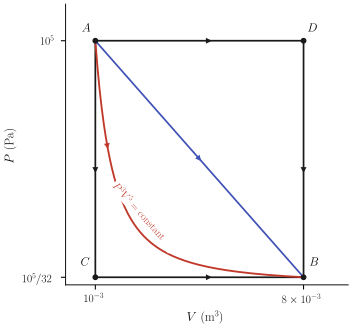
In the process \(A D B\) the gas is heated at constant pressure ( \(P=10^{5} \mathrm{~Pa}\) ) until its volume increases from its initial value of \(10^{-3} \mathrm{~m}^{3}\) to its final value of \(8 \times 10^{-3}\) \(\mathrm{m}^{3}\). The gas is then cooled at constant volume until its pressure decreases to \(10^{5} / 32 \mathrm{~Pa}\). The other processes ( \(A C B\) and \(A B\) ) can be similarly interpreted, according to the figure.
[^2]b) A small paddle is installed inside the system and is driven by an external motor (by means of a magnetic coupling through the cylinder wall). The motor exerts a torque, driving the paddle at an angular velocity \(\omega\), and the pressure of the gas (at constant volume) is observed to increase at a rate given by \[ \frac{d P}{d t}=\frac{2}{3} \frac{\omega}{V} \times \text { torque } \] Show that the energy difference of any two states of equal volumes can be determined by this process. In particular, evaluate \(U_{C}-U_{A}\) and \(U_{D}-U_{B}\).
Explain why this process can proceed only in one direction (vertically upward rather than downward in the \(P-V\) plot). c) Show that any two states (any two points in the \(P-V\) plane) can be connected by a combination of the processes in (a) and (b). In particular, evaluate \(U_{D}-U_{A}\). d) Calculate the work \(W_{A D}\) in the process \(A \rightarrow D\). Calculate the heat transfer \(Q_{A D}\). Repeat for \(D \rightarrow B\), and for \(C \rightarrow A\). Are these results consistent with those of (a)?
The reader should attempt to solve this problem before reading the following solution!
Solution a) Given the equation of the “adiabat” (for which \(Q=0\) and \(\Delta U=W\) ), we find
\[ \begin{aligned} U_{B}-U_{A} & =W_{A B}=-\int_{V_{A}}^{V_{B}} P d V=-P_{A} \int_{V_{A}}^{V_{B}}\left(\frac{V_{A}}{V}\right)^{5 / 3} d V \\ & =\frac{3}{2} P_{A} V_{A}^{5 / 3}\left(V_{B}^{-2 / 3}-V_{A}^{-2 / 3}\right) \\ & =\frac{3}{2}(25-100)=-112.5 \mathrm{~J} \end{aligned} \]
Now consider process \(A D B\) :
\[ W_{A D B}=-\int P d V=-10^{5} \times\left(8 \times 10^{-3}-10^{-3}\right)=-700 \mathrm{~J} \]
But
\[ \begin{aligned} U_{B}-U_{A} & =W_{A D B}+Q_{A D B} \\ Q_{A D B} & =-112.5+700=587.5 \mathrm{~J} \end{aligned} \]
Note that we are able to calculate \(Q_{A D B}\), but not \(Q_{A D}\) and \(Q_{D B}\) separately, for we do not (yet) know \(U_{D}-U_{A}\).
Similarly we find \(W_{A C B}=-21.9 \mathrm{~J}\) and \(Q_{A C B}=-90.6 \mathrm{~J}\). Also \(W_{A B}=-360.9\) J and \(Q_{A B}=248.4 \mathrm{~J}\). b) As the motor exerts a torque, and turns through an angle \(d \theta\), it delivers an energy \({ }^{4} d U=\) torque \(\times d \theta\) to the system. But \(d \theta=\omega d t\), so that
\[ \begin{aligned} d P & =\frac{2}{3} \frac{1}{V}(\text { torque }) \omega d t \\ & =\frac{2}{3} \frac{1}{V} d U \end{aligned} \]
or
\[ d U=\frac{3}{2} V d P \]
This process is carried out at constant \(V\) and furthermore \(d U \geq 0\) (and consequently \(d P \geq 0\) ). The condition \(d U \geq 0\) follows from \(d U=\) torque \(\times d \theta\), for the sign of the rotation \(d \theta\) is the same as the sign of the torque that induces that rotation. In particular
\[ U_{A}-U_{C}=\frac{3}{2} V\left(P_{A}-P_{C}\right)=\frac{3}{2} \times 10^{-3} \times\left(10^{5}-\frac{1}{32} \times 10^{5}\right)=145.3 \mathrm{~J} \]
and
\[ U_{D}-U_{B}=\frac{3}{2} V\left(P_{D}-P_{B}\right)=\frac{3}{2} \times 8 \times 10^{-3} \times\left(10^{5}-\frac{1}{32} \times 10^{5}\right)=1162.5 \mathrm{~J} \]
- To connect any two points in the plane we draw an adiabat through one and an isochor ( \(V=\) constant) through the other. These two curves intersect, thereby connecting the two states. Thus we have found (using the adiabatic process) that \(U_{B}-U_{A}=-112.5 \mathrm{~J}\) and (using the irreversible stirrer process) that \(U_{D}-U_{B}=\) 1162.5 J . Therefore \(U_{D}-U_{A}=1050 \mathrm{~J}\). Equivalently, if we assign the value zero to \(U_{A}\) then
\[ U_{A}=0, \quad U_{B}=-112.5 \mathrm{~J}, \quad U_{C}=-145.3 \mathrm{~J}, \quad U_{D}=1050 \mathrm{~J} \]
and similarly every state can be assigned a value of \(U\). d) Now having \(U_{D}-U_{A}\) and \(W_{A D}\) we can calculate \(Q_{A D}\).
\[ \begin{aligned} U_{D}-U_{A} & =W_{A D}+Q_{A D} \\ 1050 & =-700+Q_{A D} \\ Q_{A D} & =1750 \mathrm{~J} \end{aligned} \]
Also
\[ U_{B}-U_{D}=W_{D B}+Q_{D B} \]
or
\[ -1162.5=0+Q_{D B} \]
To check, we note that \(Q_{A D}+Q_{D B}=587.5 \mathrm{~J}\), which is equal to \(Q_{A D B}\) as found in (a).
[^3]
PROBLEMS
Problem 1.8-1
For the system considered in Example 1, calculate the energy of the state with \(P=5 \times 10^{4} \mathrm{~Pa}\) and \(V=8 \times 10^{-3} \mathrm{~m}^{3}\).
Problem 1.8-2
Calculate the heat transferred to the system considered in Example 1 in the process in which it is taken in a straight line (on the \(P-V\) diagram) from the state \(A\) to the state referred to in the preceding problem.
Problem 1.8-3
For a particular gaseous system it has been determined that the energy is given by
\[ U=2.5 P V+\text { constant } \]
The system is initially in the state \(P=0.2 \mathrm{MPa}\) (mega-Pascals), \(V=0.01 \mathrm{~m}^{3}\); designated as point \(A\) in the figure. The system is taken through the cycle of three processes ( \(A \rightarrow B, B \rightarrow C\), and \(C \rightarrow A\) ) shown in the figure. Calculate \(Q\) and \(W\) for each of the three processes. Calculate \(Q\) and \(W\) for a process from \(A\) to \(B\) along the parabola \(P=10^{5}+10^{9} \times(V-.02)^{2}\). 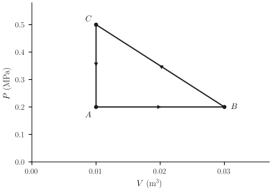
Answer:
\[ W_{B C}=7 \times 10^{3} \mathrm{~J} ; Q_{B C}=-9.5 \times 10^{3} \mathrm{~J} \]
Problem 1.8-4
For the system of Problem 1.8-3 find the equation of the adiabats in the \(P-V\) plane (i.e., find the form of the curves \(P=P(V)\) such that \(d Q=0\) along the curves).
Answer: \(V^{7} P^{5}=\) constant
Problem 1.8-5
The energy of a particular system, of one mole, is given by
\[ U=A P^{2} V \]
where \(A\) is a positive constant of dimensions \([\mathrm{P}]^{-1}\). Find the equation of the adiabats in the \(P-V\) plane.
Problem 1.8-6
For a particular system it is found that if the volume is kept constant at the value \(V_{0}\) and the pressure is changed from \(P_{0}\) to an arbitrary pressure \(P^{\prime}\), the heat transfer to the system is
\[ Q^{\prime}=A\left(P^{\prime}-P_{0}\right) \quad(A>0) \]
In addition it is known that the adiabats of the system are of the form
\[ P V^{\gamma}=\text { constant }(\gamma \text { a positive constant }) \]
Find the energy \(U(P, V)\) for an arbitrary point in the \(P-V\) plane, expressing \(U(P, V)\) in terms of \(P_{0}, V_{0}, A, U_{0} \equiv U\left(P_{0}, V_{0}\right)\) and \(\gamma\) (as well as \(P\) and \(V\) ).
Answer:
\[ U-U_{0}=A\left(P r^{\gamma}-P_{0}\right)+[P V /(\gamma-1)]\left(1-r^{\gamma-1}\right) \quad \text { where } r \equiv V / V_{0} \]
Problem 1.8-7
Two moles of a particular single-component system are found to have a dependence of internal energy \(U\) on pressure and volume given by
\[ U=A P V^{2} \quad(\text { for } N=2) \]
Note that doubling the system doubles the volume, energy, and mole number, but leaves the pressure unaltered. Write the complete dependence of \(U\) on \(P, V\), and \(N\) for arbitrary mole number.
1-9 THE BASIC PROBLEM OF THERMODYNAMICS
The preliminaries thus completed, we are prepared to formulate first the seminal problem of thermodynamics and then its solution.
Surveying those preliminaries retrospectively, it is remarkable how far reaching and how potent have been the consequences of the mere choice of thermodynamic coordinates. Identifying the criteria for those coordinates revealed the role of measurement. The distinction between the macroscopic coordinates and the incoherent atomic coordinates suggested the distinction between work and heat. The completeness of the description by the thermodynamic coordinates defined equilibrium states. The thermodynamic coordinates will now provide the framework for the solution of the central problem of thermodynamics.
There is, in fact, one central problem that defines the core of thermodynamic theory. All the ults of thermodynamics propagate from its solution.
The single, all-encompassing problem of thermodynamics is the determination of the equilibrium state that eventually results after the removal of internal constraints in a closed, composite system.
Let us suppose that two simple systems are contained within a closed cylinder, separated from each other by an internal piston. Assume that the cylinder walls and the piston are rigid, impermeable to matter, and adiabatic and that the position of the piston is firmly fixed. Each of the systems is closed. If we now free the piston, it will, in general, seek some new position. Similarly, if the adiabatic coating is stripped from the fixed piston, so that heat can flow between the two systems, there will be a redistribution of energy between the two systems. Again, if holes are punched in the piston, there will be a redistribution of matter (and also of energy) between the two systems. The removal of a constraint in each case results in the onset of some spontaneous process, and when the systems finally settle into new equilibrium states they do so with new values of the parameters \(U^{(1)}, V^{(1)}, N_{1}^{(1)} \cdots\) and \(U^{(2)}, V^{(2)}, N_{1}^{(2)} \cdots\). The basic problem of thermodynamics is the calculation of the equilibrium values of these parameters.
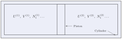
Before formulating the postulate that provides the means of solution of the problem, we rephrase the problem in a slightly more general form without reference to such special devices as cylinders and pistons. Given two or more simple systems, they may be considered as constituting a single composite system. The composite system is termed closed if it is surrounded by a wall that is restrictive with respect to the total energy, the total volume, and the total mole numbers of each component of the composite system. The individual simple systems within a closed composite system need not themselves be closed. Thus, in the particular example referred to, the composite system is closed even if the internal piston is free to move or has holes in it. Constraints that prevent the flow of energy, volume, or matter among the simple systems constituting the composite system are known as internal constraints. If a closed composite system is in equilibrium with respect to internal constraints, and if some of these constraints are then removed, certain previously disallowed processes become permissible. These processes bring the system to a new equilibrium state. Prediction of the new equilibrium state is the central problem of thermodynamics.
1.10 THE ENTROPY MAXIMUM POSTULATES
The induction from experimental observation of the central principle that provides the solution of the basic problem is subtle indeed. The historical method, culminating in the analysis of Caratheodory, is a tour de force of delicate and formal logic. The statistical mechanical approach pioneered by Josiah Willard Gibbs required a masterful stroke of inductive inspiration. The symmetry-based foundations to be developed in Chapter 21 will provide retrospective understanding and interpretation, but they are not yet formulated as a deductive basis. We therefore merely formulate the solution to the basic problem of thermodynamics in a set of postulates depending upon a posteriori rather than a priori justification. These postulates are, in fact, the most natural guess that we might make, providing the simplest conceivable formal solution to the basic problem. On this basis alone the problem might have been solved; the tentative postulation of the simplest formal solution of a problem is a conventional and frequently successful mode of procedure in theoretical physics.
What then is the simplest criterion that reasonably can be imagined for the determination of the final equilibrium state? From our experience with many physical theories we might expect that the most economical form for the equilibrium criterion would be in terms of an extremum principle. That is, we might anticipate the values of the extensive parameters in the final equilibrium state to be simply those that maximize \({ }^{5}\) some function. And, straining our optimism to the limit, we might hope that this hypothetical function would have several particularly simple mathematical properties, designed to guarantee simplicity of the derived theory. We develop this proposed solution in a series of postulates.
Postulate II. There exists a function (called the entropy \(S\) ) of the extensive parameters of any composite system, defined for all equilibrium states and having the following property: The values assumed by the extensive parameters in the absence of an internal constraint are those that maximize the entropy over the manifold of constrained equilibrium states.
It must be stressed that we postulate the existence of the entropy only for equilibrium states and that our postulate makes no reference whatsoever to nonequilibrium states. In the absence of a constraint the system is free to select any one of a number of states, each of which might also be realized in the presence of a suitable constraint. The entropy of each of these constrained equilibrium states is definite, and the entropy is largest in some particular state of the set. In the absence of the constraint this state of maximum entropy is selected by the system.
[^4]In the case of two systems separated by a diathermal wall we might wish to predict the manner in which the total energy \(U\) distributes between the two systems. We then consider the composite system with the internal diathermal wall replaced by an adiabatic wall and with particular values of \(U^{(1)}\) and \(U^{(2)}\) (consistent, of course, with the restriction that \(\left.U^{(1)}+U^{(2)}=U\right)\). For each such constrained equilibrium state there is an entropy of the composite system, and for some particular values of \(U^{(1)}\) and \(U^{(2)}\) this entropy is maximum. These, then, are the values of \(U^{(1)}\) and \(U^{(2)}\) that obtain in the presence of the diathermal wall, or in the absence of the adiabatic constraint.
All problems in thermodynamics are derivative from the basic problem formulated in Section 1.9. The basic problem can be completely solved with the aid of the extremum principle if the entropy of the system is known as a function of the extensive parameters. The relation that gives the entropy as a function of the extensive parameters is known as a fundamental relation. It therefore follows that if the fundamental relation of a particular system is known all conceivable thermodynamic information about the system is ascertainable from it.
The importance of the foregoing statement cannot be overemphasized. The information contained in a fundamental relation is all-inclusive-it is equivalent to all conceivable numerical data, to all charts, and to all imaginable types of descriptions of thermodynamic properties. If the fundamental relation of a system is known, every thermodynamic attribute is completely and precisely determined.
Postulate III. The entropy of a composite system is additive over the constituent subsystems. The entropy is continuous and differentiable and is a monotonically increasing function of the energy.
Several mathematical consequences follow immediately. The additivity property states that the entropy \(S\) of the composite system is merely the sum of the entropies \(S^{(\alpha)}\) of the constituent subsystems:
\[ S=\sum_{\alpha} S^{(\alpha)} \]
The entropy of each subsystem is a function of the extensive parameters of that subsystem alone
\[ S^{(\alpha)}=S^{(\alpha)}\left(U^{(\alpha)}, V^{(\alpha)}, N_{1}^{(\alpha)}, \ldots, N_{r}^{(\alpha)}\right) \]
The additivity property applied to spatially separate subsystems requires the following property: The entropy of a simple system is a homogeneous first-order function of the extensive parameters. That is, if all the extensive parameters of a system are multiplied by a constant \(\lambda\), the entropy is multiplied by this same constant. Or, omitting the superscript \((\alpha)\),
\[ S\left(\lambda U, \lambda V, \lambda N_{1}, \ldots, \lambda N_{r}\right)=\lambda S\left(U, V, N_{1}, \ldots, N_{r}\right) \]
The monotonic property postulated implies that the partial derivative \((\partial S / \partial U)_{V, N_{1}, \ldots, N_{r}}\) is a positive quantity,
\[ \left(\frac{\partial S}{\partial U}\right)_{V, N_{1}, \ldots, N_{r}}>0 \]
As the theory develops in subsequent sections, we shall see that the reciprocal of this partial derivative is taken as the definition of the temperature. Thus the temperature is postulated to be nonnegative. \({ }^{6}\)
The continuity, differentiability, and monotonic property imply that the entropy function can be inverted with respect to the energy and that the energy is a single-valued, continuous, and differentiable function of \(S, V, N_{1}, \ldots, N_{r}\). The function
\[ S=S\left(U, V, N_{1}, \ldots, N_{r}\right) \]
can be solved uniquely for \(U\) in the form
\[ U=U\left(S, V, N_{1}, \ldots, N_{r}\right) \]
Equations 1.8 and 1.9 are alternative forms of the fundamental relation, and each contains all thermodynamic information about the system.
We note that the extensivity of the entropy permits us to scale the properties of a system of \(N\) moles from the properties of a system of 1 mole. The fundamental equation is subject to the identity
\[ S\left(U, V, N_{1}, N_{2}, \ldots, N_{r}\right)=N S\left(U / N, V / N, N_{1} / N, \ldots, N_{r} / N\right) \]
in which we have taken the scale factor \(\lambda\) of equation 1.6 to be equal to \(1 / N \equiv 1 / \Sigma_{k} N_{k}\). For a single-component simple system, in particular,
\[ S(U, V, N)=N S(U / N, V / N, 1) \]
But \(U / N\) is the energy per mole, which we denote by \(u\).
\[ u \equiv U / N \]
[^5]Also, \(V / N\) is the volume per mole, which we denote by \(v\).
\[ v \equiv V / N \]
Thus \(S(U / N, V / N, 1) \equiv S(u, v, 1)\) is the entropy of a system of a single mole, to be denoted by \(s(u, v)\).
\[ s(u, v) \equiv S(u, v, 1) \]
Equation 1.11 now becomes
\[ S(U, V, N)=N s(u, v) \]
Postulate IV. The entropy of any system vanishes in the state for which
\[ (\partial U / \partial S)_{V, N_{1}, \ldots, N_{r}}=0 \quad \text { (that is, at the zero of temperature) } \]
We shall see later that the vanishing of the derivative \((\partial U / \partial S)_{V, N_{1}, \ldots, N_{2}}\) is equivalent to the vanishing of the temperature, as indicated. Hence the fourth postulate is that zero temperature implies zero entropy.
It should be noted that an immediate implication of postulate IV is that \(S\) (like \(V\) and \(N\), but unlike \(U\) ) has a uniquely defined zero.
This postulate is an extension, due to Planck, of the so-called Nernst postulate or third law of thermodynamics. Historically, it was the latest of the postulates to be developed, being inconsistent with classical statistical mechanics and requiring the prior establishment of quantum statistics in order that it could be properly appreciated. The bulk of thermodynamics does not require this postulate, and I make no further reference to it until Chapter 10. Nevertheless, I have chosen to present the postulate at this point to close the postulatory basis.
The foregoing postulates are the logical bases of our development of thermodynamics. In the light of these postulates, then, it may be wise to reiterate briefly the method of solution of the standard type of thermodynamic problem, as formulated in Section 1.9. We are given a composite system and we assume the fundamental equation of each of the constituent systems to be known in principle. These fundamental equations determine the individual entropies of the subsystems when these systems are in equilibrium. If the total composite system is in a constrained equilibrium state, with particular values of the extensive parameters of each constituent system, the total entropy is obtained by addition of the individual entropies. This total entropy is known as a function of the various extensive parameters of the subsystems. By straightforward differentiation we compute the extrema of the total entropy function, and then, on the basis of the sign of the second derivative, we classify these extrema as minima, maxima, or as horizontal inflections. In an appropriate physi- cal terminology we first find the equilibrium states and we then classify them on the basis of stability. It should be noted that in the adoption of this conventional terminology we augment our previous definition of equilibrium; that which was previously termed equilibrium is now termed stable equilibrium, whereas unstable equilibrium states are newly defined in terms of extrema other than maxima.
It is perhaps appropriate at this point to acknowledge that although all applications of thermodynamics are equivalent in principle to the procedure outlined, there are several alternative procedures that frequently prove more convenient. These alternate procedures are developed in subsequent chapters. Thus we shall see that under appropriate conditions the energy \(U\left(S, V, N_{1}, \ldots\right)\) may be minimized rather than the entropy \(S\left(U, V, N_{1}, \ldots\right)\), maximized. That these two procedures determine the same final state is analogous to the fact that a circle may be characterized either as the closed curve of minimum perimeter for a given area or as the closed curve of maximum area for a given perimeter. In later chapters we shall encounter several new functions, the minimization of which is logically equivalent to the minimization of the energy or to the maximization of the entropy.
The inversion of the fundamental equation and the alternative statement of the basic extremum principle in terms of a minimum of the energy (rather than a maximum of the entropy) suggests another viewpoint from which the extremum postulate perhaps may appear plausible. In the theories of electricity and mechanics, ignoring thermal effects, the energy is a function of various mechanical parameters, and the condition of equilibrium is that the energy shall be a minimum. Thus a cone is stable lying on its side rather than standing on its point because the first position is of lower energy. If thermal effects are to be included the energy ceases to be a function simply of the mechanical parameters. According to the inverted fundamental equation, however, the energy is a function of the mechanical parameters and of one additional parameter (the entropy). By the introduction of this additional parameter the form of the energyminimum principle is extended to the domain of thermal effects as well as to pure mechanical phenomena. In this manner we obtain a sort of correspondence principle between thermodynamics and mechanicsensuring that the thermodynamic equilibrium principle reduces to the mechanical equilibrium principle when thermal effects can be neglected.
We shall see that the mathematical condition that a maximum of \(S\left(U, V, N_{1}, \ldots\right)\) implies a minimum of \(U\left(S, V, N_{1}, \ldots\right)\) is that the derivative \((\partial S / \partial U)_{V, N_{1}}\),… be positive. The motivation for the introduction of this statement in postulate III may be understood in terms of our desire to ensure that the entropy-maximum principle will go over into an energyminimum principle on inversion of the fundamental equation.
In Parts II and III the concept of the entropy will be more deeply explored, both in terms of its symmetry roots and in terms of its statistical mechanical interpretation. Pursuing those inquires now would take us too far afield. In the classical spirit of thermodynamics we temporarily defer such interpretations while exploring the far-reaching consequences of our simple postulates.
PROBLEMS
Problem 1.10-1
The following ten equations are purported to be fundamental equations of various thermodynamic systems. However, five are inconsistent with one or more of postulates II, III, and IV and consequently are not physically acceptable. In each case qualitatively sketch the fundamental relationship between \(S\) and \(U\) (with \(N\) and \(V\) constant). Find the five equations that are not physically permissible and indicate the postulates violated by each.
The quantities \(v_{0}, \theta\), and \(R\) are positive constants, and in all cases in which fractional exponents appear only the real positive root is to be taken.
\(S=\left(\frac{R^{2}}{v_{0} \theta}\right)^{1 / 3}(N V U)^{1 / 3}\)
\(S=\left(\frac{R}{\theta^{2}}\right)^{1 / 3}\left(\frac{N U}{V}\right)^{2 / 3}\)
\(S=\left(\frac{R}{\theta}\right)^{1 / 2}\left(N U+\frac{R \theta V^{2}}{v_{0}^{2}}\right)^{1 / 2}\)
\(S=\left(\frac{R^{2} \theta}{v_{0}^{3}}\right) V^{3} / N U\)
\(S=\left(\frac{R^{3}}{v_{0} \theta^{2}}\right)^{1 / 5}\left[N^{2} V U^{2}\right]^{1 / 5}\)
\(S=N R \ln \left(U V / N^{2} R \theta v_{0}\right)\)
\(S=\left(\frac{R}{\theta}\right)^{1 / 2}[N U]^{1 / 2} \exp \left(-V^{2} / 2 N^{2} v_{0}^{2}\right)\)
\(S=\left(\frac{R}{\theta}\right)^{1 / 2}(N U)^{1 / 2} \exp \left(-\frac{U V}{N R \theta v_{0}}\right)\)
\(U=\left(\frac{v_{0} \theta}{R}\right) \frac{S^{2}}{V} \exp (S / N R)\)
\(U=\left(\frac{R \theta}{v_{0}}\right) N V\left(1+\frac{S}{N R}\right) \exp (-S / N R)\)
Problem 1.10-2
For each of the five physically acceptable fundamental equations in problem 1.10-1 find \(U\) as a function of \(S, V\), and \(N\).
Problem 1.10-3
The fundamental equation of system A is
\[ S=\left(\frac{R^{2}}{v_{0} \theta}\right)^{1 / 3}(N V U)^{1 / 3} \]
and similarly for system B. The two systems are separated by a rigid, impermeable, adiabatic wall. System A has a volume of \(9 \times 10^{-6} \mathrm{~m}^{3}\) and a mole number of 3 moles. System B has a volume of \(4 \times 10^{-6} \mathrm{~m}^{3}\) and a mole number of 2 moles. The total energy of the composite system is 80 J . Plot the entropy as a function of \(U_{A} /\left(U_{A}+U_{B}\right)\). If the internal wall is now made diathermal and the system is allowed to come to equilibrium, what are the internal energies of each of the individual systems? (As in Problem 1.10-1, the quantities \(v_{0}, \theta\), and \(R\) are positive constants.)